Subnetworks as Trainable Activation Functions
TL;DR: This post presents the implementation and evaluation of multilayer perceptron-based activation functions.
Introduction
In the area of machine learning, modern network architectures often use fixed activation functions such as the ReLU nonlinearity. This means that in practice we usually presume the most ideal functional form of the activation function by using predefined non-trainable nonlinearities. Due to the fixed mapping of these activation functions, there is a clear rule which signals and at what strength are allowed to pass to the next layer. However, this does not allow the network to be as flexible as it could be if the activation functions were trainable.
This post tries to explore some implications of replacing non-trainable activation functions by small fully connected neural networks. Throughout this post I will refer to these trainable activation networks as subnetworks. Multilayer perceptrons have been shown to be strong function approximators. In this context, this could prove very useful to learn more complex activation functions for better feature representation.
Related Work
Min Lin et al. used in their work on “Networks in Networks (NiN)” micro networks to replace the generalized linear model (GLM) in convolutional layers to process the input of the perceptive field by using this general nonlinear function approximator. This means that local areas in the perceptive field are mapped to the activation of the next feature map using a fully connected neural network that is shared across all patches.
One drawback of this approach, however, is that the input layer of the micro-network has the size of the perceptual field (or filter size) times the number of channels ($W \times H \times C$), which in modern network architectures leads to a large amount of additional parameters and significantly greater computational effort compared to subnetworks introduced in this post. More formally, the mapping for networks in networks can be represented by:
\[\{x_i\} \rightarrow \text{NiN} \rightarrow x_j\]In contrast to micro networks which replace the generalized linear model (GLM), subnetworks process single pre-activations coming from the GLM that already processed the receptive field. This also means that subnetworks can be used in fully connected layers. In more formal terms, for a subnetwork $s$ replacing an activation function this means:
\[\text{GLM} \rightarrow z_j \rightarrow s(z) \rightarrow x_j\]where the GLM is represented by $\sum_i x_i w_i + b_j$.
Method
The following figure shows the basic idea of a fully connected neural networks equipped with subnetworks where fixed activation functions $h(z)$ are replaced by subnetworks $s^{(l)}_i = s(z_i; w^{(l)})$. The green colored connections in the figure below is to indicate that there is only one subnetwork that is shared among all neurons of the same layer.
Subnetworks are small fully connected neural networks that are no different from ordinary densely connected networks. For computational reasons, these subnetworks consist only of a small number of neurons and a few hidden layers. Since subnetworks effectively make the network deeper, it makes sense to choose activation functions for the subnetwork that do not saturate too quickly and that are well permeable for the feedforward signal as well as the error signal during the backpropagation pass.

Since all pre-activations $z$ of a given layer are being processed by the same subnetwork $s$, it is important to ensure that the subnetwork allows a fair amount of the incoming signals to pass. This is not always the case for subnetworks using ReLU nonlinearity. If subnetworks have only a few neurons, there is a high probability that these will not be activated if for example large negative biases are learned during gradient descent. This can cause the signal transmission of the entire layer to break down during the feedforward process. Once the subnetwork ends up in this state, it is unlikely to recover, since the function’s gradient at 0 is also 0. Thus, gradient descent will not change the subnetwork’s weights anymore. One attempt to address this issue and to allow the subnetwork to recover from such a state is to equip them for example with leaky ReLUs that have a small positive gradient for negative inputs or to use for example the sine activation function.
The implementation presented in this post uses one subnetwork for each layer (see also figure above). This is a good compromise between a single subnetwork for all layers and one subnetwork for each individual neuron.
Small subnetworks consisting of two hidden layers with four hidden neurons as presented above adds only a negligible number of parameters to the network. However, it should be noted that the computational effort increases dramatically since the network’s number of activations increases eightfold.
Implementation
This section will briefly describe how subnetworks can be implemented using Tensorflow. For more detailed information about the implementation, you can find the code on Github.
Subnetworks
Replacing activation functions with an entire fully connected network is a fairly simple process with Tensorflow by overloading the layer class. This means that instead of using a simple nonlinearity, we substitute the activation function by a network that is treated as an additional layer with trainable weights and biases.
In practice in case of fully connected layers the input tensor with dimensions [batch_size, n_features] is reshaped into a single vector with dimension [batch_size * n_features]. The same also applies for convolutional layers where we reshape the input tensor’s dimensions [batch_size, feature_map_height, feature_map_width, feature_map_channels] into [batch_size * feature_map_height * feature_map_width * feature_map_channels] to be processed by the subnetwork. This approach treats every pre-activation as an independent data point. After processing the pre-activations, the subnetwork’s output (activations) will be reshaped back to the original dimensions to be processed by the next layer.
The core principle can be implemented as follows
class SubNetwork(tf.keras.layers.Layer):

   def __init__(self, conf):
       super(SubNetwork, self).__init__()
       . . .
       self.kernel = None
       self.bias = None

   def build(self, _):
       . . .

   def call(self, input_tensor):
       # Reshape input
       x = tf.reshape(tensor=input_tensor, shape=(-1, 1))

       # Feedforward pre-activation through network
       for kernel, bias in zip(self.kernel[:-1], self.bias[:-1]):
           x = tf.matmul(x, kernel) + bias
           x = self.activation_function(x)
       x = tf.matmul(x, self.kernel[-1]) + self.bias[-1]

       # Reshape back to input shape and return
       x = tf.reshape(tensor=x, shape=tf.shape(input_tensor))
       return x
Here, we receive input_tensor consisting of the network’s pre-activations which are reshaped into a single vector. The pre-activations come either from feature maps of convolutional layers or from fully connected layers.
Networks
In order to test models equipped with subnetworks against standard networks, I wrote one class to build fully connected neural networks and another to create VGG-like networks. For both models it applies that if use_subnet is True, only the activation function will be replaced by trainable subnetworks.
Multilayer Perceptron
Given a list describing the network’s layer structure and which activation function to use, the following piece of code creates a fully connected model using Keras’ functional API.
class MLP(object):

def __init__(self, conf):
   self.conf = conf
   # . . .

def build(self):
   inputs = tf.keras.layers.Input(shape=self.input_shape)
   x = tf.keras.layers.Dropout(rate=0.5)(inputs)

   if self.use_subnet:
       z = tf.keras.layers.Dense(units=self.layers_dense[0], **self.dense_config)(x)
       x = SubNetwork(self.conf)(z) #+ z
   else:
       x = tf.keras.layers.Dense(units=self.layers_dense[0], activation=self.activation_function,
                                 **self.dense_config)(x)
   x = tf.keras.layers.Dropout(rate=0.5)(x)

   for units in self.layers_dense[1:]:
       if self.use_subnet:
           z = tf.keras.layers.Dense(units=units, **self.dense_config)(x)
           x = SubNetwork(self.conf)(z) #+ z
       else:
           x = tf.keras.layers.Dense(units=units, activation=self.activation_function, **self.dense_config)(x)
       x = tf.keras.layers.Dropout(rate=0.5)(x)

   outputs = tf.keras.layers.Dense(self.n_classes)(x)
   model = tf.keras.Model(inputs=inputs, outputs=outputs, name="mlp")
   return model
Convolutional Neural Network
The convolutional neural network class follows the same logic and creates a model using Keras’ functional API. Two lists describe the network’s convolutional and fully connected layer structure. An additional parameter defines which activation function the CNN will use if use_subnet evaluates to False.
class CNN(object):

   def __init__(self, conf):
       # . . .

   def build(self):
       inputs = tf.keras.layers.Input(shape=self.input_shape)
       x = inputs

       # Convolutional part
       for filters in self.units_conv:
           x = self.conv_block(x, filters)
       x = tf.keras.layers.Flatten()(x)

       # Dense part
       for units in self.units_dense:
           x = tf.keras.layers.Dense(units=units, **self.conf_dense)(x)
           if self.use_subnet:
               x = SubNetwork(self.conf)(x)
           else:
               x = self.activation_function(x)
       x = tf.keras.layers.Dense(units=self.n_classes, **self.conf_dense)(x)

       model = tf.keras.models.Model(inputs=inputs, outputs=x)
       return model

   def conv_block(self, inputs, filters):
       x = tf.keras.layers.Conv2D(filters=filters, **self.conf_conv)(inputs)
       if self.use_subnet:
           x = SubNetwork(self.conf)(x)
       else:
           x = self.activation_function(x)

       x = tf.keras.layers.Conv2D(filters=filters, **self.conf_conv)(x)
       if self.use_subnet:
           x = SubNetwork(self.conf)(x)
       else:
           x = self.activation_function(x)

       x = tf.keras.layers.MaxPool2D(**self.conf_pool)(x)

       return x
Experiments
There are many aspects that make subnetworks very interesting. Here, two of these aspects will be examined in more detail:
- How does the use of subnetworks affect the model’s performance?
- What kind of activation functions are actually learned by subnetworks?
For the experiments two simple network types are used. A fully connected neural network and a VGG-like convolutional neural network. Both networks consist of eight hidden layers.
The network specifications for the MLP are as follows:
network:
 type: "mlp"
 units_dense: [1024, 1024, 1024, 1024, 1024, 1024, 1024, 1024]
 activation_function: "leaky_relu"
The following parameters were selected for the CNN:
network:
 type: "cnn"
 units_conv: [32, 64, 128]
 units_dense: [256, 256]
 activation_function: "leaky_relu"
For both networks above the following two subnetworks with three hidden layers and four neurons per layer with leaky ReLUs and sine activation functions have been used.
subnetwork:
 use_subnet: True
 units: [1, 4, 4, 4, 1]
 activation_function: "leaky_relu"
subnetwork:
 use_subnet: True
 units: [1, 4, 4, 4, 1]
 activation_function: "sin"
Fully connected networks have been trained on the Fashion-MNIST dataset for 250 epochs at a constant learning rate of 3e-4 using the Adam optimizer and a batch size of 1024. The dropout rate was set to 0.5 for subnetworks with sine activation functions and 0.2 for subnetworks using leaky ReLUs.
Convolutional neural networks have also been trained on the Fashion-MNIST dataset. Due to the much larger number of pre-activations in convolutional layers resulting in a much higher computational load and memory usage, the number of training epochs was reduced to 100 with a batch size of 128. The learning rate was set to 3e-4, and dropout applied to the densely connected part of the network was chosen to be 0.5.
For the evaluation of both experiments, the results of 10 runs were averaged.
Results
Multilayer Perceptron
Below are the results for networks equipped with subnetworks using leaky ReLU and sine activation functions compared to the baseline network with fixed nonlinearity.
Leaky ReLU Subnetworks


Sine Subnetworks


It is noticeable that the networks’ loss and accuracy are less volatile if equipped with fixed non-trainable activation functions. The picture is different for network’s equipped with subnetworks. Here the variance of loss and accuracy between several runs is much higher. It is interesting to see that in some cases these networks significantly outperform the baseline model in terms of accuracy.
It is notable that after 250 epochs, models equipped with subnetworks using sine activation functions dominate in terms of training accuracy and training loss. The network equipped with subnetworks using leaky ReLUs dominated only on the training data and was after 250 epochs on par with the standard network on the validation data. The validation costs suggest that stronger regularization could have been used in training. Interestingly, leaky ReLU subnetworks could only be trained with smaller dropout rates.
Details of the performance comparison are shown in the following tables.
| Activation Function | Training Accuracy | Validation Accuracy |
|---|---|---|
| Leaky ReLU | 0.9013 $\pm$ 0.0007 | 0.8924 $\pm$ 0.0015 |
| Subnetwork (Leaky ReLU) | 0.9222 $\pm$ 0.0022 | 0.8928 $\pm$ 0.0027 |
| Activation Function | Training Accuracy | Validation Accuracy |
|---|---|---|
| Leaky ReLU | 0.8614 $\pm$ 0.0007 | 0.8699 $\pm$ 0.0026 |
| Subnetwork (Sine) | 0.8828 $\pm$ 0.0036 | 0.8888 $\pm$ 0.0024 |
Both figures below show the resulting graphs of individual subnetworks equipped with leaky ReLU and sine activation functions in different layers. The functions’ definition range was chosen such that about 99.7% of the pre-activations entering the subnetwork are within three standard deviations.
Leaky ReLU Subnetworks Graphs

Sine Subnetworks Graphs

Both figures show that there is no emerging pattern for the subnetwork in the same layer. Very different activation functions are learned during each run. Furthermore, it seems that there aren’t any noticeable differences between the functions learned by the subnetwork in different layers.
Convolutional Neural Network
Below are the results for convolutional neural networks combined with subnetworks equipped with leaky ReLU and sine activation functions compared to the baseline network with non-trainable nonlinearities.
Leaky ReLU Subnetworks


Sine Subnetworks

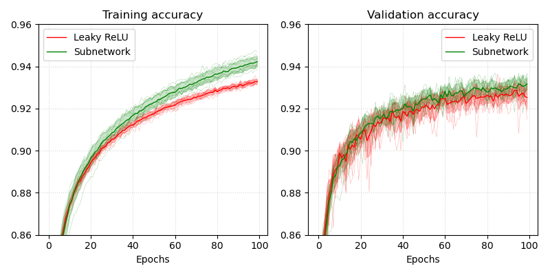
It is interesting to see that when activation functions are replaced by subnetworks, they perform significantly better on the training data, despite the small number of additional parameters. On the other hand, both networks perform about the same on validation data after 100 epochs.
Details of the performance comparison are shown in the following tables.
| Activation Function | Training Accuracy | Validation Accuracy |
|---|---|---|
| Leaky ReLU | 0.9323 $\pm$ 0.0013 | 0.928 $\pm$ 0.0036 |
| Subnetwork (Leaky ReLU) | 0.9444 $\pm$ 0.0063 | 0.9328 $\pm$ 0.0052 |
| MethActivation Function | Training Accuracy | Validation Accuracy |
|---|---|---|
| Leaky ReLU | 0.9327 $\pm$ 0.0001 | 0.9252 $\pm$ 0.0054 |
| Subnetwork (Sine) | 0.9422 $\pm$ 0.0025 | 0.9316 $\pm$ 0.0031 |
The following two figures show that also in the case of CNNs, there are no recurring patterns for subnetworks in the same layer. Very different activation functions are learned during each run.
Leaky ReLU Subnetworks Graphs

Sine Subnetworks Graphs

Discussion
The results show that using subnetworks rather than standard activation functions have the potential to outperform classic network architectures. This could be due to the fact that trainable activation functions may increase the network’s overall ability of feature representations.
A major disadvantage of subnetworks is, of course, the large amount of computation required to train these kinds of networks. Depending on the network type in the experiments above, networks needed two to three times as much time to train. At this point it also remains unknown what the ideal size of a subnetwork with respect to the parent network is, which activation function should be used, and what a good initialization scheme for the subnetwork’s weight is.
Since adding subnetworks to a model basically adds many additional layers to the network, these kinds of networks are no longer easy to train. This problem could be addressed by adding shortcut connections that bypass the subnetworks.
It is also notable that subnetworks only increase the network’s performance if they are combined with dropout. This suggests that other regularization techniques may also have a strong influence on the performance growth that is added by subnetworks.
It is also interesting to note that networks equipped with subnetworks can be trained with larger learning rates. This could be due to the fact that subnetworks lead to smaller gradients more quickly, which is possibly compensated for by larger learning rates.
Outlook
Despite the increased computational complexity of adding subnetworks to neural networks, the results provide evidence that these kinds of networks can outperform classical network architectures, where high-speed inference is not essential.
I hope to see future studies where subnetworks are used in much larger networks, as this is probably the only way to determine their true value.
@misc{Fischer2021laf,
  title={Subnetworks as Trainable Activation Functions},
  author={Fischer, Kai},
  howpublished={\url{https://kaifishr.github.io/2021/02/02/learning-activation-functions.html}},
  year={2021}
}
You find the code for this project here.