A Multilayer Perceptron with NumPy
TL;DR: A simple Python implementation of a fully connected feedforward artificial neural network designed to help you get a better feel for these types of machine learning algorithms. This post provides the implementation as well as the underlying maths. The MNIST and Fashion-MNIST datasets are used to check the correctness of the implementation.
Introduction
In this blog post I’ll show how to implement a simple multilayer perceptron neural network (or simply MLP) in Python using the numerics library NumPy. The network uses NumPy’s highly optimized matrix multiplication functions and is therefore relatively fast to train. This low-level implementation (in Python terms) of a multilayer perceptron is easily accessible and allows to understand the underlying mechanisms of simple neural networks. At the same time it might destroy the magic around this topic a little bit as you will realize, that it is just some simple linear algebra and analysis that bring such a network to life. Multilayer perceptrons can process any abstract vector space representation of data, i.e., any data you can represent as an vector of numbers.
Implementation
This implementation of a neural network uses ReLU activation functions as non-linearities in its hidden layers. The network’s error is computed by first applying the sigmoid activation function to the network’s output neurons before the L2 loss was computed.
Notation
The network is implemented in Python as a class. For the sake of better readability, I removed all the self terms in the following code snippets.
Network initialization
The networks structure is defined by a python tuple consisting the number of neurons of the network’s input, hidden, and output layer. Thus
network_config = (n_input, 128, 128, 128, n_classes)
represents a five-layered network (network_depth = len(network_config)), that consists of three hidden layers of 128 neurons each. Next, we initialize the network’s trainable parameters, that is its weights W and biases b:
# Weights
W = [kaiming(network_config, l) for l in range(network_depth-1)]
# Biases
b = [np.zeros((network_config[l], 1)) for l in range(1, network_depth)]
Initialization of Trainable Parameters
An adequate weight initialization scheme is a crucial part before training deep neural networks as it often helps the model to converge faster. Weight initialization prevents activations from becoming too big or too small during the feedforward pass. During the error backpropagation process, both situations will either lead to gradients that are too large or to small and thus prevent the network from converging (due to disappearing or exploding gradients).
This implementation uses a method proposed by Kaiming He et al. to initialize the weights. The weights of layer l are drawn from a normal distribution with zero mean and standard deviation of \(\sqrt{\frac{2}{n_l}}\), i.e.,
Biases are set to zero. This initialization scheme can be implemented in Python as follows
def kaiming(network_config, l):
    return np.random.normal(size=(network_config[l+1], network_config[l])) \
           * np.sqrt(2./network_config[l])
Activation Functions
In the following, the activation functions’ definitions, derivatives and implementations are shown. The rectifier activation function is defined as the positive part of its argument. In scientific publications, different notations of this activation function can be found:
\[\text{ReLU(z)} = z^+ = \max(z,0) = \frac{1}{2}(|z|+z)\]def relu(z):
return z[z<0]
with its derivative
\[\frac{\partial \text{ReLU(z)}}{\partial z} = H(z) = \frac{1}{2}(\frac{z}{|z|}+1)\]where \(H(z)\) is the Heaviside function.
def relu_prime(z):
    return (z>0).astype(x.dtype)
The sigmoid activation function is defined by the formula
\[\sigma(z) = \frac{1}{1+e^{-z}}\]def sigma(z):
return expit(z)
with its derivative
\[\frac{\partial \sigma(z)}{\partial z} = \sigma(z)(1-\sigma(z))\]def sigma_prime(z):
u = sigma(z)
return u-u*u
Feedforward
The feedforward operation is a fairly simple process that consists of successive matrix-vector multiplications. It uses the list of weights and biases from the last section to transform the network’s input data in a nonlinear fashion projecting it to the output neurons. For a single neuron with index \(i\) in layer \((l+1)\), this process can be formulated as follows
\[z_i^{(l+1)} = \sum_{j=1}^{n_{l}} w_{ij}^{(l+1,l)} a_j^{(l)} + b_i^{(l+1)}\] \[a_i^{(l+1)} = h (z_i^{(l+1)})\]Here, \(z_i^{(l+1)}\), also referred to as pre-activation, represents the result of a linear affine transformation of the input \(a_j^{(l)}\). The weigth \(w_{ij}^{(l+1,l)}\) connects neurons \(i\) and \(j\) of the adjacent layers \((l+1)\) and \((l)\). The number of neurons in layer \(l\) is given by \(n_l\). In a next step, the pre-activation is transformed by a nonlinear activation function \(h(\cdot)\) resulting in the neuron’s activation \(a_j^{(l+1)}\). This implementation uses the Rectified Linear Unit \(\text{ReLU}(\cdot)\) activation function for the hidden layer neurons and the sigmoid activation function \(\sigma(\cdot)\) at the output layer. The resulting implementation of the feedforward pass in Python can be written in a very compact form:
def feedforward(X):
    a[0] = X
    for l in range(network_depth-2):
        z[l] = np.matmul(a[l], W[l].T) + .b[l].T
        a[l+1] = relu(z[l])
    z[-1] = np.matmul(a[-2], W[-1].T) + b[-1].T
    a[-1] = sigma(z[-1])
Loss computation
After feedforwarding the data, the network’s output activations \(a_i^{(L)}\) are compared to the true label \(y_i\). That is, we measure the distance between the network’s output and the target value using a pre-defined loss function (or cost function). Here, we use the L2 loss
\[C = \frac{1}{2}\sum_{i=1}^{n_{L}} (a_i^{(L)} - y_i)^2\]which measures the Euclidean distance between the network’s output and the true label. The added constant factor \(\frac{1}{2}\) leads to nicer looking terms when calculating the gradients in the next step. This loss function oftentimes is used in regression tasks but also serves as a candidate for multi-class classification tasks. In Python, the L2 loss can be implemented as follows
loss = ((a[-1] - Y)**2).sum()
Backpropagation Gradient Descent
Now that we have defined a loss function we can backpropagate the error signal to adjust the weights and biases in the network. For this implementation of a multilayer perceptron, the weights and biases of the network are optimized using a very basic form of mini-batch stochastic gradient descent, which is an iterative optimization scheme to improve the network’s performance over time. The term stochastic comes from the fact that the gradient descent algorithm uses a random batch of samples out of the training data during every optimization step.
The following implementation of the gradient descent algorithm consists of two main parts. First the gradients are being computed by doing a backward pass through the network. In the second step, the computed gradients are being used to update the network’s weights and biases. Let’s start with the first step, the backpropagation process.
Output Layer
In the following, we derive the backpropagation gradient descent formulas for a single input (batch size equals one). We start at the network’s output layer \(L\) where the error is being computed. Let’s look at the network’s loss function, the output’s preactivations and activations:
\[C = \frac{1}{2}\sum_{i=1}^{n_{L}} (a_i^{(L)} - y_i)^2\] \[z_i^{(L)} = \sum_{j=1}^{n_{L-1}} w_{ij}^{(L,L-1)} a_j^{(L-1)} + b_j^{(L)}\] \[a_i^{(L)} = \sigma (z_i^{(L)})\]Now we can use the chain rule of calculus to compute the weight’s impact on the loss function. Or to put it another way, how does a change of a weight in our network affect the loss. We do this for both, the weights that connect the last hidden layer neurons to the output layer neurons and the output layer’s biases:
\[\frac{\partial C}{\partial w_{ij}^{(L,L-1)}} = \frac{\partial C}{\partial a_i^{(L)}} \cdot \frac{\partial a_i^{(L)}}{\partial z_i^{(L)}} \cdot \frac{\partial z_i^{(L)}}{\partial w_{ij}^{(L,L-1)}} = (a_i^{(L)} - y_i) \cdot \sigma'(z_i^{(L)}) \cdot a_j^{(L-1)}\] \[\frac{\partial C}{\partial b_i^{(L)}} = \frac{\partial C}{\partial a_i^{(L)}} \cdot \frac{\partial a_i^{(L)}}{\partial z_i^{(L)}} \cdot \frac{\partial z_i^{(L)}}{\partial b_i^{(L)}} = (a_i^{(L)} - y_i) \cdot \sigma'(z_i^{(L)})\]Let’s translate this into vectorized code for arbitrary batch size:
delta = (a[-1] - Y) * sigma_prime(z[network_depth-2])
dW[network_depth-2] += delta.T.dot(a[network_depth-2])
db[network_depth-2] += np.sum(delta.T, axis=1, keepdims=True)
Hidden Layer
In the last section we have seen how to compute the gradients to adjust the weights that connect the last hidden layer to the output layer. Now we derive the formula to compute the gradients for the weights that connect hidden layer \((l)\) to hidden layer \((l-1)\). Starting from the hidden layer neurons in layer \((l)\)
\[z_j^{(l)} = \sum_{k=1}^{n_{l-1}} w_{jk}^{(l,l-1)} a_k^{(l-1)} + b_j^{(l)}\] \[a_j^{(l)} = h(z_j^{(l)})\]where \(h(\cdot)\) stands for the activation function, the gradients are computed as follows
\[\frac{\partial C}{\partial w_{jk}^{(l,l-1)}} = \frac{\partial z_j^{(l)}}{\partial w_{jk}^{(l,l-1)}} \cdot \frac{\partial a_j^{(l)}}{\partial z_j^{(l)}} \cdot \frac{\partial C}{\partial a_j^{(l)}} = a_k^{(l-1)} \cdot h'(z_j^{(l)}) \cdot \frac{\partial C}{\partial a_j^{(l)}}\] \[\frac{\partial C}{\partial b_j^{(l)}} = \frac{\partial z_j^{(l)}}{\partial b_j^{(l)}} \cdot \frac{\partial a_j^{(l)}}{\partial z_j^{(l)}} \cdot \frac{\partial C}{\partial a_j^{(l)}} = h'(z_j^{(l)}) \cdot \frac{\partial C}{\partial a_j^{(l)}}\]with
\[\frac{\partial C}{\partial a_j^{(l)}} = \sum_{i=1}^{n_{l+1}} \frac{\partial z_i^{(l+1)}}{\partial a_j^{(l)}} \cdot \frac{\partial a_i^{(l+1)}}{\partial z_i^{(l+1)}} \cdot \frac{\partial C}{\partial a_i^{(l+1)}}\]A vectorized version of the equations above can be written in a very compact way
for l in reversed(range(network_depth-2)):
    delta = delta.dot(W[l+1]) * relu_prime(z[l])
    dW[l] += a[l].T.dot(delta).T
    db[l] += np.sum(delta.T, axis=1, keepdims=True)
Gradient Descent
Now that we have computed all the gradients during the backpropagation process, we can use these gradients to adjust the network’s weights and biases. For a weight \(w\) connecting two neurons the update rule is as follows
\[w^{(t+1)} = w^{(t)} - \eta \cdot \frac{\partial C}{\partial w^{(t)}}\]where \(w^{(t)}\) and \(w^{(t+1)}\) represent the old and the updated weight, respectively. The same update rule applies to the network’s biases. The learning rate of the algorithm is given by \(\eta\). Translating this into code and we get
for l in range(network_depth-1):
    W[l] -= eta * dW[l]
    b[l] -= eta * db[l]
After completing a gradient descent step, the computed gradients are reseted for the next optimization step. Putting it all together, we get:
def backprop_gradient_descent(Y, eta):
    # Error backpropagation and gradient computation
    delta = (a[-1] - Y) * sigma_prime(z[network_depth-2])
    dW[network_depth-2] += delta.T.dot(a[network_depth-2])
    db[network_depth-2] += np.sum(delta.T, axis=1, keepdims=True)

    for l in reversed(range(network_depth-2)):
        delta = delta.dot(W[l+1]) * relu_prime(z[l])
        dW[l] += a[l].T.dot(delta).T
        db[l] += np.sum(delta.T, axis=1, keepdims=True)

    # Gradient descent: Update Weights and Biases
    for l in range(network_depth-1):
        W[l] -= eta * dW[l]
        b[l] -= eta * db[l]

    # Reset gradients for next optimization step
    dW = [np.zeros_like(dW[l]) for l in range(network_depth-1)]
    db = [np.zeros_like(db[l]) for l in range(network_depth-1)]
Methods
We will test the performance of this implementation using the MNIST and the Fashion-MNIST dataset as these allow some nice visualizations of what the network has learned during training. To test the network’s performance, a three-layered network with 128 neurons per hidden layer was trained for 200 epochs using a constant learning rate of 0.2, and a mini-batch size of 64. 10% of the training data were used as a validation set during the training run. The images’ gray-scale pixel values were linearly normalized to range from -1 to 1 instead of 0 to 255 using the following formula
\[I \leftarrow 2 \cdot \frac{I - I_{\text{min}}}{I_{\text{max}} - I_{\text{min}}} - 1\]which can be implemented as follows
def normalization(I):
    return 2*(I/255.0 - 0.5)
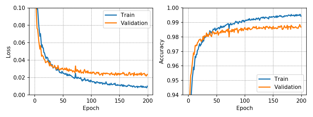
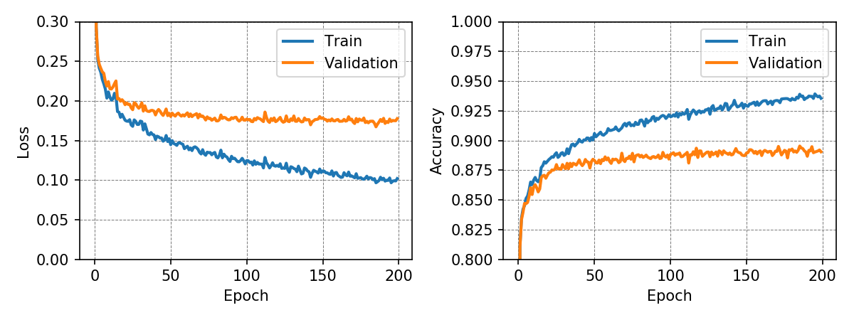
Results
The following graphs show loss and accuracy for the training and validation dataset. The network achieved a test accuracy of 98.50% and 88.81% for the MNIST and Fashion-MNIST dataset, respectively.
To understand a little bit better what is going on inside a neural network, the weights connecting the input to the first hidden layer can be visualized.
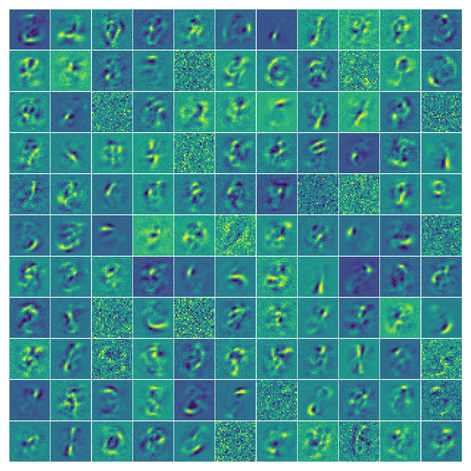
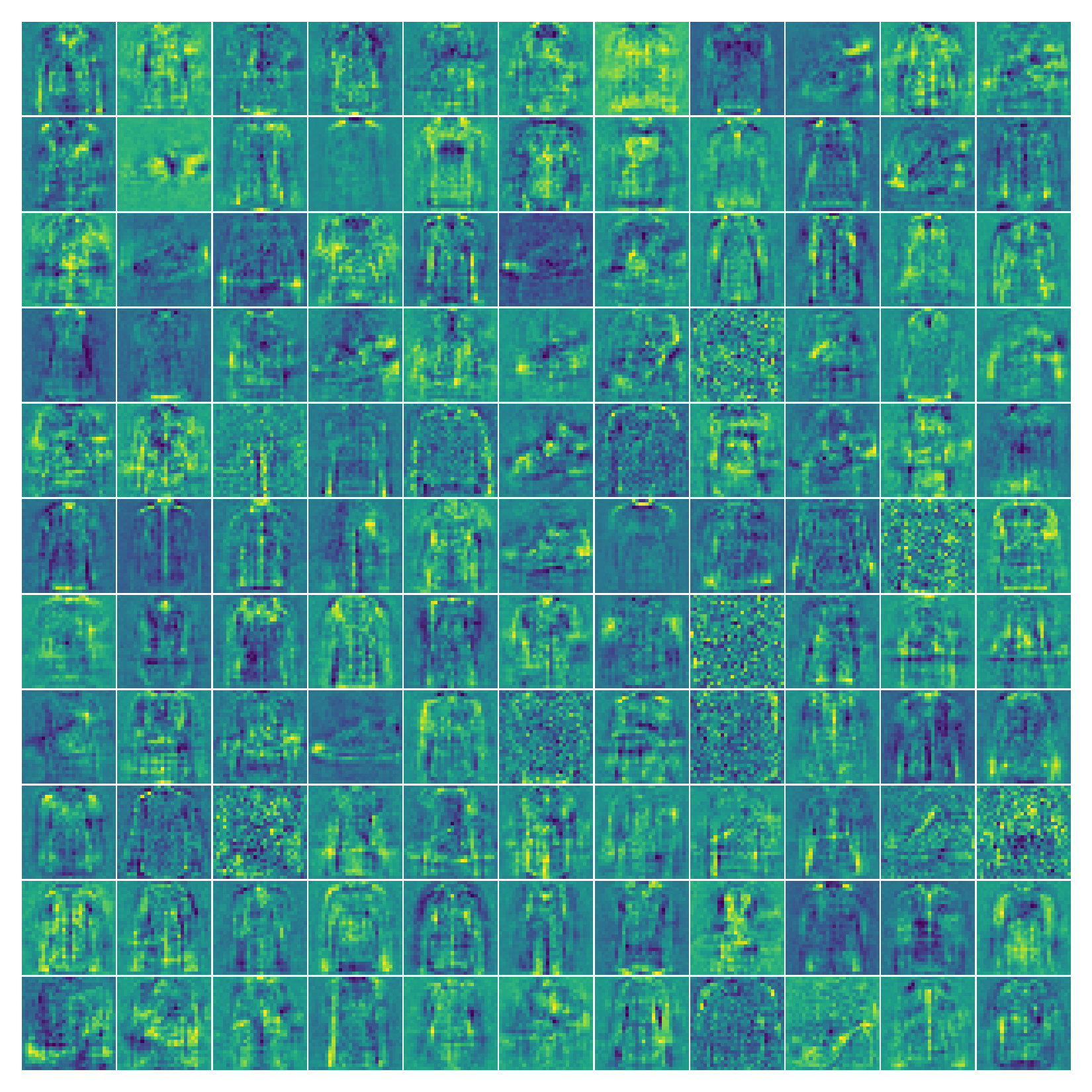
It is interesting to see, that the neural network learns filters that can amplify and suppress characteristics of certain classes. The visualization of the weights also shows, that some neurons may not contribute a great deal to the classification as their associated filters consist almost exlusively of noise.
Discussion
This project is a very basic implementation of a fully connected neural network with many possibilities for improvement such as L2 regularization, dropout, batch normalization, softmax cross-entropy loss, to name but a few. The network can easily be modified to address regression problems or can be converted to an autoencoder with almost no effort. The results for the three-layered fully connected neural network show good performance for the MNIST and Fashion-MNIST dataset. The weight visualization gives a rough clue which features of the input images are of particular importance for a network to map its input to the correct output.
The complete code of the project can be found here.