Training a Simple Classifier using an Evolutionary Algorithm
TL;DR: A linear multi-class classification model can be trained relatively quickly using an evolutionary algorithm and can reach 91.77% (MNIST) and 83.72% (Fashionin-MNIST) of test accuracy.
Introduction
This post is about multi-class classification with linear regression. Despite the fact that this problem can be efficiently solved analytically or by using a gradient descent optimization algorithm, this post shows that it is possible to train such a classifier using genetic optimization.
Usually, genetic optimization of such a model is much slower compared to other optimization techniques that take advantage of the property, that the loss function is differentiable with respect to its weights. The resulting optimization schemes such as an analytical solution or gradient descent are able to optimize small models pretty quickly. However, genetic algorithms are an amazingly interesting topic as they can be applied very easily to a wide range of problems including non-differential models 1 or discrete optimization.
Methods
To demonstrate what a multi-class linear classification model trained with an evolutionary algorithm is capable of, I am using the MNIST and Fashion-MNIST datasets which consist of grayscale images with 28 x 28 pixles. For this model, each pixel is associated with a weight parameter. Both datasets consist of 10 classes and each class is assigned a bias term. Thus, there is a total number of 28 x 28 x 10 + 10 = 7850 trainable parameters. The set of all weights can be considered as the chromosome that evolves during the optimization process and the single weights as genes. The set of all chromosomes represent the population size. The words chromosomes, individuals and agents are used interchangeably.
The two main optimization processes, that imitate fundamental properties of evolution, are the mutation and chromosome crossover operations. While mutation operations act on all members of a population, the crossover operations are only applied to the n fittest members of a population that are then passed to the next generation.
The following list shows how a genetic algorithm for this type of problem is usually structured:
- Generate an initial population consisting of weight matrices
- Evaluate the fitness of each individual by computing its loss
- Select the
nbest individuals - Perform crossover operations on these individuals and duplicate the result
- Generate random mutations on these new individuals and return to step 2
The implementation discussed here, varies slightly from the description above. Since the implementation makes use of Python’s multiprocessing library that allows optimizing one population per CPU core, the optimization process is performed for local_epochs on several cores in parallel. This means, that these populations do not interact (do not exchange genes) for local_epochs. This has the effect that different populations can develop different strengths during this time. After local_epochs periods the best candidates of each population are being compared with each other. The chromosomes of the top two candidates then undergo the crossover operation resulting in a new prototype that is then scattered across all cores. This process is repeated for global_epochs periods.
Both, the mutation and crossover operations can be implemented very easily. For a given weight matrix W out of the chromosome pool, the mutation operations can be implemented as follows
def mutation(W):
    W = W + mutation_rate*np.random.uniform(-1, 1, size=W.shape) \
        * (np.random.random(size=W.shape) < update_probability)
    return W
Here, mutation_rate can be compared to the learning rate of a gradient descent optimizer and specifies how strongly a gene is mutated. On the other hand, update_probability determines how likely it is for a gene to be changed and thus also controls the number of weights being updated in each training step.
The crossover operation takes the weight matrices of two individuals, W_1 and W_2, recombines them and returns a new weight matrix. The following implementation demonstrates uniform crossover where genes of both individuals are randomly selected and combined to form a new chromosome.
def crossover(W_1, W_2):
    B_1 = np.random.randint(2, size=W_1.shape)
    return B_1*W_1 + (1-B_1)*W_2
This implementation of the crossover operation gives each gene a 50% chance to become part of the new gene pool.
Training
Before training the model, pixel values of each image were rescaled into a range of [-1,1]. A total of 10% of the training data was used as validation set. Furthermore, the error was computed by first applying the softmax function to the classifier’s output before the L2 loss was computed to determine the fittest agent.
Parameters
To train the classifier, the following parameters were used during the optimization process:
batch_size = 16
local_epochs = 10
global_epochs = 100
mutation_rate = 0.001
update_probability = 0.01
local_population_size = 4
global_population_size = 4
Where local_population_size represents the number of agents on every core and global_population_size represents the number of individual populations. The mutation rate, which acts on the gene level, and the update probability, which acts on the chromosome level, were chosen to be small in order to mimic evolutionary processes which are very slowly.
Results
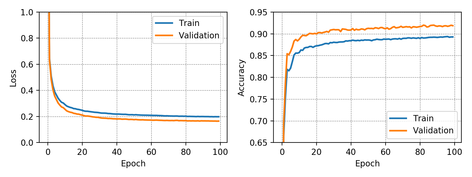
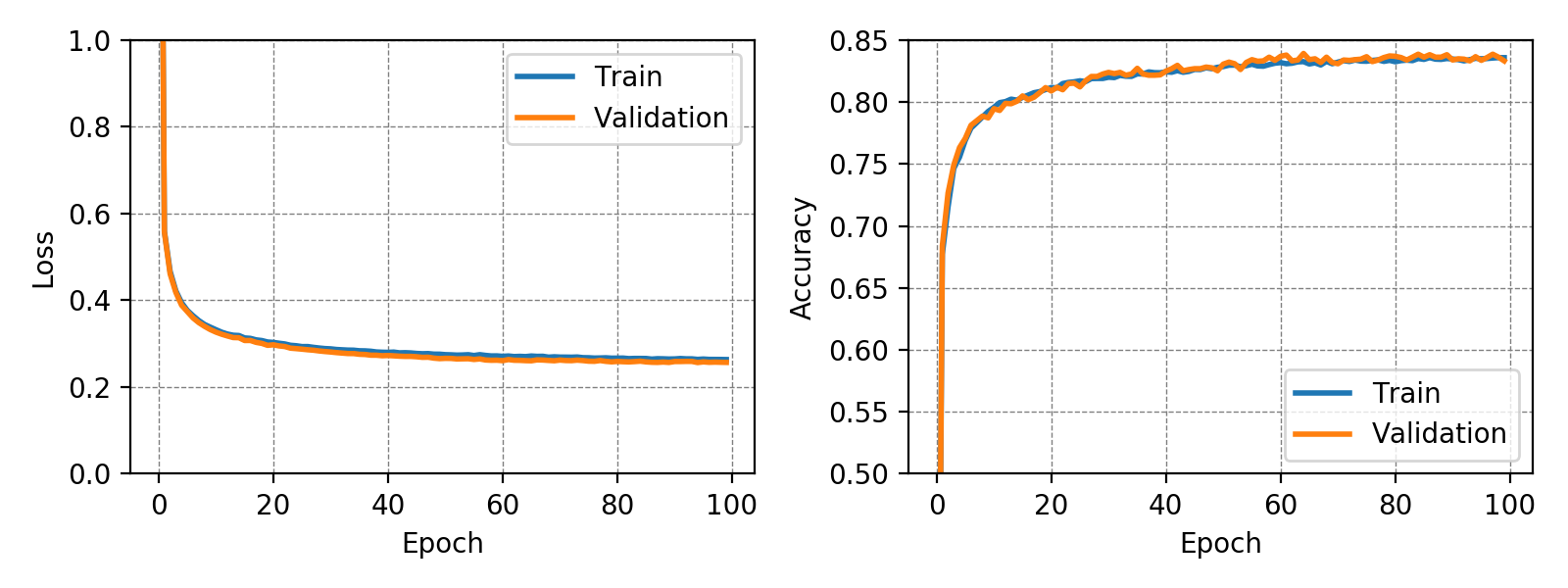
The classifier trained on the MNIST dataset achieved a test accuracy of 91.77% while the classifier trained on the more complex Fashion-MNIST dataset achieved a test accuracy of 83.72%. In both training runs no overfitting could be observed. This may have been due to the very small number of trainable parameters. It is interesting to note, that for the MNIST dataset the validation accuracy is constantly higher than the training accuracy. The following graphs show loss and accuracy for the validation and test set of the MNIST and Fashion-MNIST dataset.
In case of the Fashion-MNIST dataset there is almost no difference between the results of the training and validation set.
The weights for every class can also be visualized and help to understand what the classifier has learned during the training process of 100 global epochs.
Discussion
The results showed that simple classification tasks can be solved to a certain degree with genetic optimization. Despite the fact that the accuracy of the model is far from state-of-the-art, after all, the results are not that bad for a genetic optimizer and a light weight model that consists of only 7850 weights. It is worth mentioning that logistic regression models that were trained using a gradient descent optimizer achieved similar results (see here and here). These models achieved a test accuracy of about 91% and 84% for the MNIST and the Fashion-MNIST dataset, respectively.
The visualization of the weights in the course of 100 epochs reveals, how the models evolved and that they learned to give greater weight to important and more unqiue features of the individual classes in order to distinguish them from other classes. It is exciting to see that this smart behaviour results from such a simple set of rules.
Conclusion
Training a simple classifier with a genetic optimization scheme is possible and yields similar results compared to approaches that use a gradient descent optimizer or the analytic solution. However, genetic optimization takes much more time and is generally not recommended for such a task. More complex models, such as deep neural networks, that consist of multiple layers will be even more difficult to train with such an approach. However, since genetic optimization does not depend on gradients it is possible to train small multi-layered neural networks that use activation functions whose derivate is zero such as the Heaviside step function. For this reason it might be interesting and worth taking a look in this direction.
The complete code of the project can be found here.
-
Such as an artifical neural network that uses Heaviside activation functions. ↩