An Adaptive Learning Rate Method for Gradient Descent Algorithms

TL;DR: Gradient information can be used to compute adaptive learning rates that allow gradient descent algorithms to converge much faster.

Introduction

In this blog post I present an adaptive learning rate method for gradient descent optimization algorithms. To the best of my knowledge, this method has not yet been mentioned in the literature.

The proposed technique uses gradient information that allow to either compute parameter-wise or global adaptive learning rates. In more detail, the learning rate is treated as a differentiable function allowing to propagate the loss information back so that the learning rate can be adjusted accordingly.

The method can easily be applied to popular optimization algorithms such as Gradient Descent, Gradient Descent with Momentum, Nestrov Accelerated Gradient, or Adam, to name just a few. In a few simple experiments I show, that these optimization algorithms show better performance when equipped with the adaptive learning rate method introduced in this post compared to their standard implementation.

In recent years many learning rate schedules have been proposed that work on top of optimizers to improve the training of machine learning models. Most of these methods have in common, that they do not take information such as the loss or gradient information into account that is provided by the model during the training process.

The learning rates of some of these methods approach very small values at the end of training such as learning rate methods with exponential decay or one-cycle learning rate policies. However, such learning rate policies are not very plausible from a biological point of view since the model will not learn new information as well at the end of training as it did at the beginning of training when the learning rate was higher. Such small learning rates prevent the model from reaching better local minima if new information is available. Therefore, these methods work best for a fixed set of data that does not change during training.

For this reason, cyclic learning rate policies may be the better option for continuous learning. However, also in the case of cyclic learning rate schedules, it can be hard to find optimal parameters such as the minimal and maximal learning rate or the period length of one cycle.

To avoid the problem of specifiying an additional learning rate schedule, optimizers such as Adam, AdaGrad, AdaDelta, or RMSprop adaptively change the step size to take larger gradient descent steps in shallow and small steps in steep directions by tracking both, the gradient as well as the second moment of the gradient. In practice, however, even these optimizers are often equipped with an additional learning rate policy to improve the result. But this leads to the same problems as just described.

To overcome the need of specifiying a learning rate schedule manually, we can use the gradient information provided by the model itself to compute an adaptive learning rate at every optimization step. This will be the main contribution of this blog post.

Method

In this section we derive an adaptive learning rate update scheme for gradient descent optimization algorithms. Stochastic gradient descent computes the gradient of a loss function $L$ with respect to the parameters $w$. The update rule for each parameter can be written as follows:

\begin{equation} \label{eq:weight_update} w_i^{(t+1)} = w_i^{(t)} - \eta_{i}^{(t)} \frac{dL^{(t)}}{dw_i^{(t)}} \end{equation}

We assume that we can backpropagate the loss information to the learning rate $\eta$ to adapt the learning rate for the subsequent weight update. For parameter-wise learning rates this can be written as follows:

\begin{equation} \label{eq:learning_rate_update} \eta_{i}^{(t)} = \eta_{i}^{(t-1)} - \alpha \frac{dL^{(t)}}{d\eta_{i}^{(t-1)}} \end{equation}

Where $\alpha$ is a newly introduced hyperparameter determining the rate of change of the adaptive learning rate. We can expand the last term of Equation \eqref{eq:learning_rate_update} using the chain rule of calculus and get

\begin{equation}\label{eq:dLdeta} \frac{dL^{(t)}}{d\eta_{i}^{(t-1)}} = \frac{dL^{(t)}}{dw_{i}^{(t)}}\frac{dw_{i}^{(t)}}{d\eta_{i}^{(t-1)}} \end{equation}

Now we can use Equation \eqref{eq:weight_update} to rewrite the right-hand side of Equation \eqref{eq:dLdeta} such that it only consists of gradients of the loss with respect to the weights. Taking the derivate of Equation \eqref{eq:weight_update} with respect to the learning rate $\eta$ we get

\begin{equation}\label{eq:dwdeta} \frac{dw_{i}^{(t)}}{d\eta_{i}^{(t-1)}} = -\frac{dL^{(t-1)}}{dw_{i}^{(t-1)}} \end{equation}

By substituting the last term of Equation \eqref{eq:dLdeta} with the result of Equation \eqref{eq:dwdeta} we get:

\begin{equation}\label{eq:dLdeta_2} \frac{dL^{(t)}}{d\eta_{i}^{(t-1)}} = -\frac{dL^{(t)}}{dw_i^{(t)}}\frac{dL^{(t-1)}}{dw_{i}^{(t-1)}} \end{equation}

Now Equation \eqref{eq:dLdeta_2} can be inserted into Equation \eqref{eq:learning_rate_update} to get the final result which is an update rule that allows to compute parameter-wise adaptive learning rates

\begin{equation}\label{eq:learning_rate_update_2} \eta_{i}^{(t)} = \eta_{i}^{(t-1)} + \alpha \frac{dL^{(t)}}{dw_i^{(t)}}\frac{dL^{(t-1)}}{dw_{i}^{(t-1)}} \end{equation}

Here, we can make several interesting observations. The update rule uses the gradients of the current and last time step to determine the next learning rate.

The product of the old and the new gradient allows for two different cases. If both gradients are either positive or negative, the result is positive resulting in an increase of the learning rate for the next weight update. This seems to make sense since subsequent gradients with the same sign indicate that there is a clear direction within the loss landscape and that the error is probably moving towards a local minimum.

On the other hand, successive gradients with different signs may indicate that there is no clear direction for the gradient descent in the loss landscape. In this case, the product of both gradients is negative causing the learning rate for the considered parameter to decrease. At this point it is important to note that this method allows the learning rate to become negative. Decreasing the learning rate allows a more careful gradient descent or even an ascent if the learning rater becomes negative. This may be beneficial to escape from local minima.

By inserting Equation \eqref{eq:learning_rate_update_2} into Equation \eqref{eq:weight_update} we obtain the following expression for the weight update rule with adaptive learning rate:

\begin{equation}\label{eq:weight_update_2} w_i^{(t+1)} = w_i^{(t)} - \eta_{i}^{(t-1)} \frac{dL^{(t)}}{dw_i^{(t)}} - \alpha \left(\frac{dL^{(t)}}{dw_{i}^{(t)}} \right)^2 \frac{dL^{(t-1)}}{dw_{i}^{(t-1)}} \end{equation}

As can be seen, the newly introduced parameter $\alpha$ determines the effect of the correction term on the weight update.

It is also possible to derive an update scheme for a learning rate $\eta^{(t)}$ that is the same for all parameters. In this case we pool the gradient information of all parameters to compute a single global learning rate. To do this, we can write the last term of Equation \eqref{eq:learning_rate_update} as follows

\begin{equation}\label{eq:dLdeta_global} \frac{dL^{(t)}}{d\eta^{(t-1)}} = \frac{1}{||\Omega||} \sum_{i \in \Omega} \frac{dL^{(t)}}{dw_{i}^{(t)}}\frac{dw_{i}^{(t)}}{d\eta^{(t-1)}} \end{equation}

Where $\Omega$ denotes the model’s set of trainable parameters. Please note that at this point the index $i$ is no longer needed for the learning rate. Thus, we write $\eta^{(t)}$ instead of $\eta_{(i)}^{(t)}$. We now insert the result of Equation \eqref{eq:dwdeta} into Equation \eqref{eq:dLdeta_global} to get:

\begin{equation}\label{eq:dLdeta_global_2} \frac{dL^{(t)}}{d\eta^{(t-1)}} = - \frac{1}{||\Omega||} \sum_{i \in \Omega} \frac{dL^{(t)}}{dw_{i}^{(t)}}\frac{dL^{(t-1)}}{dw_{i}^{(t-1)}} \end{equation}

By inserting Equation \eqref{eq:dLdeta_global_2} into Equation \eqref{eq:learning_rate_update} we get the update rule for a global learning rate.

\begin{equation}\label{eq:learning_rate_update_global} \eta^{(t)} = \eta^{(t-1)} + \alpha \frac{1}{||\Omega||} \sum_{i \in \Omega} \frac{dL^{(t)}}{dw_{i}^{(t)}}\frac{dL^{(t-1)}}{dw_{i}^{(t-1)}} \end{equation}

We can now insert Equation \eqref{eq:learning_rate_update_global} into Equation \eqref{eq:weight_update} to obtain the weight update rule for a global adaptive learning rate:

\begin{equation}\label{eq:weight_update_global} w_i^{(t+1)} = w_i^{(t)} - \eta^{(t-1)}\frac{dL^{(t)}}{dw_i^{(t)}} - \frac{\alpha}{||\Omega||}\frac{dL^{(t)}}{dw_i^{(t)}} \sum_{j \in \Omega} \frac{dL^{(t)}}{dw_{j}^{(t)}}\frac{dL^{(t-1)}}{dw_{j}^{(t-1)}} \end{equation}

Implementation

In this section I show how the method introduced above can be integrated into common gradient descent optimization algorithms. The implementation is fairly straightforward and can also be found on my Github repository.

First, we define the test function. In this case Beale’s function:

def f(x, y):
    """
    Beale's function
    """
    return (1.5 - x + x*y)**2 + (2.25 - x + x*y**2)**2 + (2.625 - x + x*y**3)**2

Next, the partial derivatives with respect to $x$ and $y$ are implemented. Here I use a simple implementation of the difference quotient (see here for more stable versions of the difference quotient) in order to be able to also use other test functions.

def dfdx(x, y, h=1e-9):
    return 0.5 * (f(x+h, y) - f(x-h, y)) / h

def dfdy(x, y, h=1e-9):
    return 0.5 * (f(x, y+h) - f(x, y-h)) / h

The next step is to implement the standard gradient descent. Here the learning rate $\eta$ is constant for the entire optimization process.

eta_x = eta 
eta_y = eta 

def gradient_descent():
    x -= eta * dfdx(x, y)
    y -= eta * dfdy(x, y)

Given the gradient descent optimizer as implemented above, we can now add the adaptive learning rate method to the algorithm by caching the new gradients to determine the new learning rate based on the last two gradients and then performing gradient descent. Afterwards, the new gradients are cached for the next optimization step.

def gradient_descent():
    dx = dfdx(x, y)
    dy = dfdy(x, y)

    eta_x += alpha * dx * dx_old
    eta_y += alpha * dy * dy_old

    x -= eta_x * dx
    y -= eta_y * dy

    dx_old = dx
    dy_old = dy

The next example shows the integration of an adaptive learning rate for the Adam optimizer. The implementation steps are the same.

def gradient_descent_adam():
    dx = dfdx(x, y)
    dy = dfdy(x, y)

    m_x = beta_1 * m_x_old + (1.0 - beta_1) * dx
    m_y = beta_1 * m_y_old + (1.0 - beta_1) * dy

    v_x = beta_2 * v_x_old + (1.0 - beta_2) * dx * dx
    v_y = beta_2 * v_y_old + (1.0 - beta_2) * dy * dy

    m_x_hat = m_x / (1.0 - beta_1**(i+1))
    m_y_hat = m_y / (1.0 - beta_1**(i+1))

    v_x_hat = v_x / (1.0 - beta_2**(i+1))
    v_y_hat = v_y / (1.0 - beta_2**(i+1))

    eta_x += alpha * dx * dx_old
    eta_y += alpha * dy * dy_old

    x -= (eta_x / (np.sqrt(v_x_hat) + epsilon)) * m_x_hat
    y -= (eta_y / (np.sqrt(v_y_hat) + epsilon)) * m_y_hat

    m_x_old = m_x
    m_y_old = m_y

    v_x_old = v_x
    v_y_old = v_y

    dx_old = dx
    dy_old = dy

Experiments

Now we want to perform some experiments that allow us to compare popular gradient descent optimization algorithms such as Gradient Descent (GD), Gradient Descent with Momentum (GDM), Nestrov Accelerated Gradient (NAG), and Adam with and without the parameters-wise adaptive learning rate. Optimizers equipped with an adaptive learning rate method are marked by a plus sign (GD+, GDM+, NAG+, Adam+).

To better understand the behavior of these methods we can visualize the gradient descent using a popular test function (see also here for more such functions) for optimization algorithms such as Beale’s function:

\[f(x,y) = (1.5 - x + xy)^2 + (2.25 - x + xy^2)^2 + (2.625 - x + xy^3)^2\]

In order to determine an optimal learning rate $\eta$ as well as the hyperparameter $\alpha$ for each optimizer, a grid search was performed beforehand. The optimal hyperparameter is determined by how fast the global minimum is reached. To measure the speed of convergence of different optimizers I used a loss function that is defined as the Euclidean distance to the global minimum.The following table shows the used hyperparameters:

Hyperparameter	GD	GD+	GDM	GDM+	NAG	NAG+	Adam	Adam+
$\eta$	0.01	0.01	0.015	0.01	0.006	0.006	0.0005	0.0005
$\alpha$	0	1e-4	0	1e-5	0	1e-6	0	1e-8

Please note, that the initial learning rate for all optimizers with adaptive learning rate are equal or smaller compared to the standard algorithm. For other hyperparameters, frequently used values found in the literature were used:

$\gamma=0.5$, $\beta_1=0.9$, $\beta_2=0.99$, $\epsilon=1e-8$

Results

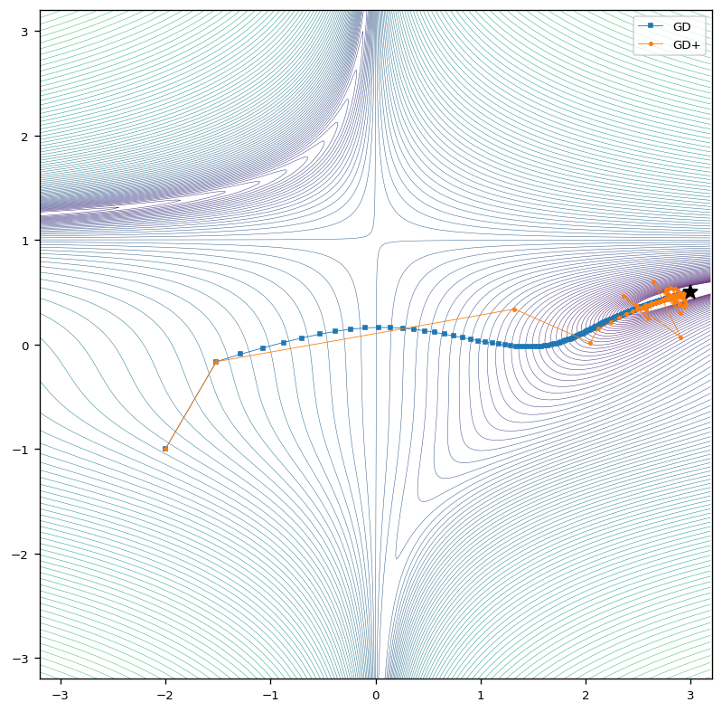
For better comparability, results are shown for one optimizer at a time. Beale’s function has a global minimum at $(x,y)=(3,0.5)$ which is indicated by a black star in the results section.

Gradient Descent

The following figure shows the behavior of the classic Gradient Descent (GD) algorithm. We see that the algorithms equipped with an adaptive learning rate (GD+) approaches the global minimum on a similar path but with much larger steps. Near the global minimum, larger oscillations are observed at the beginning of the optimization for the optimizer with adaptive learning rate.

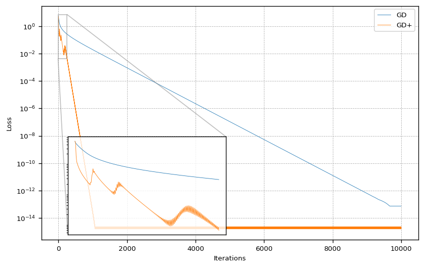
This behavior is also reflected in the loss as the next figure shows. The loss shows that the adaptive learning rate not only allows to approach the global minimum much faster, it also gets about an order of magnitude closer after convergence.

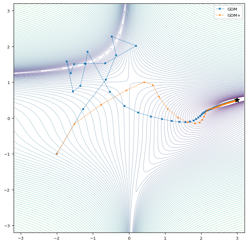
Gradient Descent with Momentum

In the case with momentum, the results behave similarly to those for the classic gradient descent. The optimizer with adaptive learning rates reaches the global minimum in a more direct way and and with larger steps.

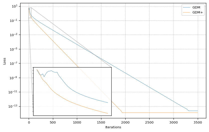
Here we see again, that the optimizer equipped with an adaptive learning rate converges much faster and also gets closer to the global minimum.

Nestrov Accelerated Gradient

In case of the Nestrov Accelerated Gradient (NAG) optimizer with a fixed learning rate, the optimizer approaches the global minimum more carefully compared to the method equipped with an adaptive learning rate. Here we see that NAG+ again behaves more aggressive right at the beginning of the optimization process.

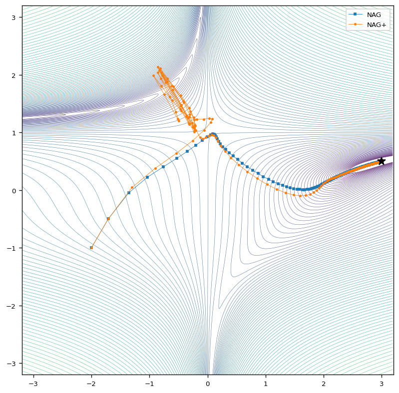
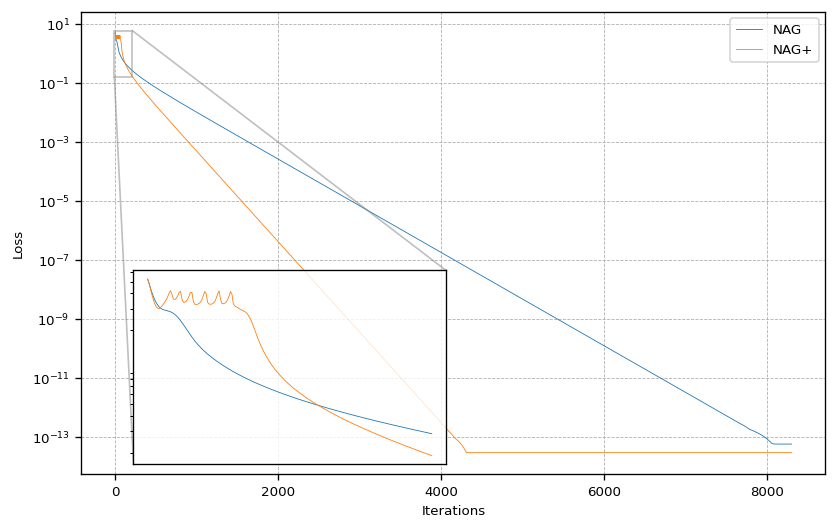
Even thought the gradient descent with NAG+ does not approach the minimum right from the start, it converges with a slight delay much faster requiring only about half the steps to converge compared to NAG.

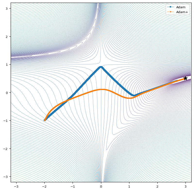
Adam

The next figure shows the results for the Adam optimization algorithm. The results show that the Adam algorithm with constant learning rate approaches to global minimum in a steady and very carefully way. If we equip the Adam optimizer with a parameter-wise adaptive learning rate, we observe, that the gradient descent is again much more aggressive, which means that the global minimum is approached with larger steps and in a more direct way.

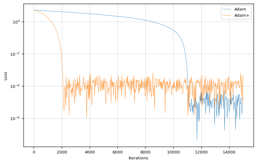
By looking at the loss we see how much faster the optimizer with adaptive learning rate converges. Interestingly, even though standard Adam takes much for time to converge, it gets closer to the global minimum by about one order of magnitude.

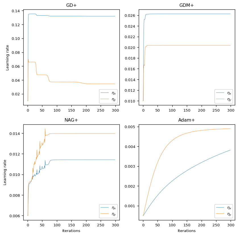
Visualization of Adaptive Learning Rates

The following figure shows the learning rates $\eta_x$ and $\eta_y$ for each optimizer used in the experiments. Visualizing the adaptive learning rates shows, how the learning rates are subject to major changes, especially at the beginning of the optimization process. In all experiments, the learning rates converged towards a certain step size.

Discussion

The single most striking observation to emerge from the experimental results was, that the global minimum is reached much faster for optimizers equipped with the adaptive learning rate presented above. It is also noteworthy, that in most cases, an adaptive learning rate also resulted in a smaller error after convergence.

As the visualization of the learning rates has shown, there is a sharp increases right at the beginning of the optimization process, probably caused due to large gradients of the test function. In the further course, the learning rate then adapts to the topological conditions before it then converges towards a certain value. The convergence results from the fact that the gradients become very small when the global minimum is reached.

Outlook

I showed that a new gradient-based method for adaptive learning rates can significantly increase the performance of popular gradient descent optimization algorithms such as GD, GDM, NAG or Adam. Not only do these optimizers equipped with the adaptive learning rate converge much faster, in most cases they also get much closer to the global minimum in the experiments.

In a next step, this method should be applied to a larger machine learning model to better assess its actual performance and its advantages and disadvantages. Furthermore, one could investigate which initial values for the parameter $\alpha$ is reasonable and how numerical stability of the method can be guaranteed.

@misc{Fischer2020alrm,
  title={An Adaptive Learning Rate Method for Gradient Descent Algorithms},
  author={Fischer, Kai},
  howpublished={\url{https://kaifishr.github.io/2020/12/18/adaptive-learning-rate-method.html}},
  year={2020}
}

You find the code for this project here.

Hyperparameter	GD	GD+	GDM	GDM+	NAG	NAG+	Adam	Adam+
\(\eta\)	0.01	0.01	0.015	0.01	0.006	0.006	0.0005	0.0005
\(\alpha\)	0	1e-4	0	1e-5	0	1e-6	0	1e-8