A Multilayer Perceptron in C++
TL;DR: This post presents the derivation and implementation of the stochastic gradient descent algorithm applied to a three-layered multilayer perceptron in C++.
Introduction
This post serves as an introduction to the working horse algorithm in deep learning, the backpropagation (stochastic) gradient descent algorithm, and shows how this algorithm can be implemented in C++. Throughout this post, a multilayer perceptron network with three hidden layers serves as an example. For better understanding, the derivation of the algorithm and the implementation is explicitly focused on a three-layered network, but can be generalized later without much effort. A simple classification task is used to test the implementation.
Method
The implementation of a fully connected neural network can be divided into two parts. The feedforward part, that consists of the mapping from input to output space, and the backpropagation gradient descent part, where the network actually learns.
In a multilayer perceptron, the feedforward process, i.e. the mapping of information from the input to the output dimension, consists of many affine transformations followed by nonlinear transformations.
\begin{equation} \label{eq:affinetransformation} \underbrace{z = \sum_i w_i x_i + b}_{\text{Affine transformation}} \end{equation}
\begin{equation} \label{eq:nonlineartransformation} \underbrace{x = h(z)}_{\text{Nonlinear transformation}} \end{equation}
The following visualization of the three-layered fully connected neural network should contribute to a better understanding of the derivation below and the subsequent implementation.
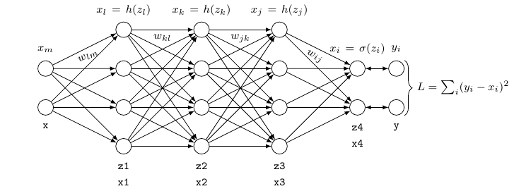
For our three layer neural network, the mapping can be formulated as follows, starting at the network’s input layer:
Input $\rightarrow$ Hidden 1
\begin{equation} \label{eq:z1} z_l = \sum_m w_{lm} x_m + b_l \end{equation}
\begin{equation} \label{eq:x1} x_l = h(z_l) \end{equation}
Hidden 1 $\rightarrow$ Hidden 2
\begin{equation} \label{eq:z2} z_k = \sum_l w_{kl} x_l + b_k \end{equation}
\begin{equation} \label{eq:x2} x_k = h(z_k) \end{equation}
Hidden 2 $\rightarrow$ Hidden 3
\begin{equation} \label{eq:z3} z_j = \sum_k w_{jk} x_k + b_j \end{equation}
\begin{equation} \label{eq:x3} x_j = h(z_j) \end{equation}
Hidden 3 $\rightarrow$ Output
\begin{equation} \label{eq:z4} z_i = \sum_j w_{ij} x_j + b_i \end{equation}
\begin{equation} \label{eq:x4} x_i = \sigma(z_i) \end{equation}
Here, $h(\cdot)$ represents some activation function such as the rectified linear (ReLU), that transforms its input in a nonlinear fashion, $\sigma(\cdot)$ represents the activation function at the network’s final layer that maps the output to the interval between 0 and 1, and $x_i$ stands for the network’s final neuron-wise prediction at the output layer.
After successfully mapping the input signal to the network’s output, the error of the prediction can be determined. For this purpose, one can make use of the simple L2 loss function, which is defined as follows
\begin{equation} \label{eq:loss_function} L = \frac{1}{2} \sum_i (y_i - x_i)^2 \end{equation}
where $y_i$ represents the true label that the network is trying to predict.
Now that we have described the feedforward process as well as the computation of the loss, we can use the information gathered during the feedforward process, i.e. the network’s activations and preactivations, to compute the gradients for all weights and biases in our network. This is also the first part to derive an optimization algorithm that allows us to train our network.
In contrast to the feedforward process, we now start at the network’s output and work our way back to the input layer. Since the loss function is a multiple nested function, we can use the chain rule of calculus to compute the desired gradients.
We start by looking at how the weights connecting the last two layers affect the loss function.
\[\begin{equation} \begin{gathered} \label{eq:gradients4} \frac{dL}{dw_{ij}} &=& \frac{dz_i}{dw_{ij}} \cdot \frac{dx_i}{dz_i} \cdot \frac{dL}{dx_i}\\ &=& x_j \cdot \underbrace{h'(z_i) \cdot (x_i - y_i)}_{\delta_i} \end{gathered} \end{equation}\]The gradients for the biases are determined analogously.
\[\begin{equation} \begin{gathered} \label{eq:gradients4b} \frac{dL}{db_{i}} &=& \frac{dz_i}{db_{i}} \cdot \frac{dx_i}{dz_i} \cdot \frac{dL}{dx_i}\\ &=& 1 \cdot \underbrace{h'(z_i) \cdot (x_i - y_i)}_{\delta_i} \end{gathered} \end{equation}\]These are already the first two rules that tell us how to compute the gradients for all weights $w_{ij}$ and biases $b_i$. As can be seen in Equation \eqref{eq:gradients4} and \eqref{eq:gradients4b}, the expressions are almost identical except for the first term. For this reason, the explicit derivation of the gradients for the biases will be omitted in the following. Here, I also identified the last two terms in Equation \eqref{eq:gradients4} and \eqref{eq:gradients4b} with $\delta_i$. Later on, this allows us to compute the gradients in a much more efficient way.
Now that we have determined the first gradients, we can proceed to the calculation of the gradients for the weights and biases connecting the last two hidden layers. Since from now on each weight and bias influences the activity of all deeper layer neurons, it must be taken into account that the error signals for each individual weight and bias must be summed up.
\[\begin{equation} \begin{gathered} \label{eq:gradients3} \frac{dL}{dw_{jk}} &=& \frac{dz_j}{dw_{jk}} \cdot \frac{dx_j}{dz_j} \cdot \sum_i \frac{dz_i}{dx_j} \cdot \frac{dx_i}{dz_i} \cdot \frac{dL}{dx_i}\\ &=& x_k \cdot \underbrace{h'(z_j) \cdot \sum_i w_{ij} \cdot \overbrace{h'(z_i) \cdot (x_i - y_i)}^{\delta_i}}_{\delta_j} \end{gathered} \end{equation}\] \[\begin{equation} \begin{gathered} \label{eq:gradients3b} \frac{dL}{db_{j}} &=& \frac{dz_j}{db_{j}} \cdot \frac{dx_j}{dz_j} \cdot \sum_i \frac{dz_i}{dx_j} \cdot \frac{dx_i}{dz_i} \cdot \frac{dL}{dx_i}\\ &=& 1 \cdot \underbrace{h'(z_j) \cdot \sum_i w_{ij} \cdot \overbrace{h'(z_i) \cdot (x_i - y_i)}^{\delta_i}}_{\delta_j} \end{gathered} \end{equation}\]Equation \eqref{eq:gradients3} shows that certain terms, marked by a $\delta$ occur repeatedly during the gradient calculation. This can be exploited in the implementation in order to avoid calculating certain quantities over and over again.
Let’s now have a look at the weights connecting the first two hidden layers. We can compute the gradients in the same fashion, and we’ll see that a repeating patter occurs.
\[\begin{equation} \begin{gathered} \label{eq:gradients2} \frac{dL}{dw_{kl}} &=& \frac{dz_k}{dw_{kl}} \cdot \frac{dx_k}{dz_k} \cdot \sum_j \frac{dz_j}{dx_k} \cdot \frac{dx_j}{dz_j} \cdot \sum_i \frac{dz_i}{dx_j} \cdot \frac{dx_i}{dz_i} \cdot \frac{dL}{dx_i}\\ &=& x_l \cdot h'(z_k) \cdot \sum_j w_{jk} \cdot \underbrace{h'(z_j) \cdot \sum_i w_{ij} \cdot \overbrace{h'(z_i) \cdot (x_i - y_i)}^{\delta_i}}_{\delta_j}\\ &=& x_l \cdot \underbrace{h'(z_k) \cdot \sum_j w_{jk} \delta_j}_{\delta_k} \end{gathered} \end{equation}\] \[\begin{equation} \begin{gathered} \label{eq:gradients2b} \frac{dL}{db_{k}} &=& \frac{dz_k}{db_{k}} \cdot \frac{dx_k}{dz_k} \cdot \sum_j \frac{dz_j}{dx_k} \cdot \frac{dx_j}{dz_j} \cdot \sum_i \frac{dz_i}{dx_j} \cdot \frac{dx_i}{dz_i} \cdot \frac{dL}{dx_i}\\ &=& 1 \cdot h'(z_k) \cdot \sum_j w_{jk} \delta_j \end{gathered} \end{equation}\]Finally, we can now compute the gradients for the weights connecting the input to the first hidden layer.
\[\begin{equation} \begin{gathered} \label{eq:gradients1} \frac{dL}{dw_{lm}} &=& \frac{dz_l}{dw_{lm}} \cdot \frac{dx_l}{dz_l} \cdot \sum_k \frac{dz_k}{dx_l} \cdot \frac{dx_k}{dz_k} \cdot \sum_j \frac{dz_j}{dx_k} \cdot \frac{dx_j}{dz_j} \cdot \sum_i \frac{dz_i}{dx_j} \cdot \frac{dx_i}{dz_i} \cdot \frac{dL}{dx_i}\\ &=& x_m \cdot \underbrace{h'(z_l) \cdot \sum_k w_{kl} \cdot h'(z_k) \cdot \sum_j w_{jk} \cdot \underbrace{h'(z_j) \cdot \sum_i w_{ij} \cdot \overbrace{h'(z_i) \cdot (x_i - y_i)}^{\delta_i}}_{\delta_j}}_{\delta_l}\\ &=& x_m \cdot \underbrace{h'(z_l) \cdot \sum_k w_{kl} \delta_k}_{\delta_l} \end{gathered} \end{equation}\] \[\begin{equation} \begin{gathered} \label{eq:gradients1b} \frac{dL}{db_{l}} &=& 1 \cdot h'(z_l) \cdot \sum_k w_{kl} \delta_k \end{gathered} \end{equation}\]In Equation \eqref{eq:gradients1} it is interesting to see, how the error signal from the network’s output is carried all the way back to the weights connecting the first two layers of our network.
The only thing missing now is the gradient descent by updating the weights and biases using the gradients that we have just computed:
\[\begin{equation} \begin{gathered} \label{eq:update4} w_{ij}^{(t+1)} = w_{ij}^{(t)} - \eta \cdot \frac{dL}{dw_{ij}^{(t+1)}} , \qquad b_{i}^{(t+1)} = b_{i}^{(t)} - \eta \cdot \frac{dL}{db_{i}^{(t+1)}} \end{gathered} \end{equation}\] \[\begin{equation} \begin{gathered} \label{eq:update3} w_{jk}^{(t+1)} = w_{jk}^{(t)} - \eta \cdot \frac{dL}{dw_{jk}^{(t+1)}} , \qquad b_{j}^{(t+1)} = b_{j}^{(t)} - \eta \cdot \frac{dL}{db_{j}^{(t+1)}} \end{gathered} \end{equation}\] \[\begin{equation} \begin{gathered} \label{eq:update2} w_{kl}^{(t+1)} = w_{kl}^{(t)} - \eta \cdot \frac{dL}{dw_{kl}^{(t+1)}} , \qquad b_{k}^{(t+1)} = b_{k}^{(t)} - \eta \cdot \frac{dL}{db_{k}^{(t+1)}} \end{gathered} \end{equation}\] \[\begin{equation} \begin{gathered} \label{eq:update1} w_{lm}^{(t+1)} = w_{lm}^{(t)} - \eta \cdot \frac{dL}{dw_{lm}^{(t+1)}} , \qquad b_{l}^{(t+1)} = b_{l}^{(t)} - \eta \cdot \frac{dL}{db_{l}^{(t+1)}} \end{gathered} \end{equation}\]Here I have marked the current training iteration by $()^{(t+1)}$. The learning rate is given by $\eta$. Now that we are able to compute the necessary gradients to train our network, we can move on to the next section where we’re going to implement the equations derived above.
Implementation
This section will roughly outline the implementation of the algorithm above in C++. In this section I will not go into detail about the generation of synthetic datasets in detail, but only into the core algorithm that is used to train the network. You can find all the code for this project on Github.
Weight Initialization
Using a good weight initialization scheme is crucial as it often helps the network to converge significantly faster and also allows for much deeper network architectures. To initialize the network’s weights connecting the neurons of adjacent layers, the He initialization turned out to be very useful. See also here. The network’s biases are initialized with zero.
void NeuralNetwork::he_initialization(std::vector<std::vector<double>>& W) {
    double mean = 0.0;
    double std = std::sqrt(2.0 / static_cast<double>(W.size()));
    std::normal_distribution<double> rand_normal(mean, std);
    for (unsigned int i=0; i<W.size(); ++i) {
        for (unsigned int j=0; j<W[0].size(); ++j) {
            W[i][j] = rand_normal(gen);
        }
    }
}
Activation Functions
The network uses two different types of activation functions. The rectified linear unit (ReLU) in the hidden layers of the network, and the sigmoid function at the network’s output. The ReLU function for the feedforward pass and its derivative for the backward pass can be implemented in C++ as follows
std::vector<double> NeuralNetwork::relu(const std::vector<double>& z) {
    std::vector<double> x(z.size());
    for (unsigned int i=0; i<z.size(); ++i) {
        if (z[i] > 0.0) {
            x[i] = z[i];
        } else {
            x[i] = 0.0;
        }
    }
    return x;
}
double NeuralNetwork::relu_prime(const double z) {
    double x;
    if (z >= 0.0) {
        x = 1.0;
    } else {
        x = 0.0;
    }
    return x;
}
At the network’s output layer, we use the sigmoid function to squeeze the preactivations into the range between 0 and 1. In order to avoid numerical overflow while using the sigmoid function we can implement a numerically stable version of it. We do this by separating large negative or large positive preactivations.
std::vector<double> NeuralNetwork::sigmoid(const std::vector<double>& z) {
    std::vector<double> x(z.size());
    for (unsigned int i=0; i<z.size(); ++i) {
        if (z[i] > 0.0) {
            x[i] = 1.0 / (1.0 + std::exp(-z[i]));
        } else {
            x[i] = std::exp(z[i]) / (1.0 + std::exp(z[i]));
        }
    }
    return x;
}
double NeuralNetwork::sigmoid_prime(const double z) {
    double sigma;
    if (z > 0.0) {
        sigma = 1.0 / (1.0 + std::exp(-z));
    } else {
        sigma = std::exp(z) / (1.0 + std::exp(z));
    }
    return sigma * (1.0 - sigma);
}
Feedforward
The feedforward() method uses the activation functions shown above and the matmul() operation that also processes the bias.
void NeuralNetwork::feedforward() {
    z1 = matmul(W1, x, b1);
    x1 = relu(z1);
    z2 = matmul(W2, x1, b2);
    x2 = relu(z2);
    z3 = matmul(W3, x2, b3);
    x3 = relu(z3);
    z4 = matmul(W4, x3, b4);
    x4 = sigmoid(z4);
}
The matmul() operation performs an affine transformation of its input x using the weights W and biases b of the corresponding layer and returns the preactivations z.
std::vector<double> NeuralNetwork::matmul(const std::vector<std::vector<double>>& W,
                                          const std::vector<double>& x,
                                          const std::vector<double>& b) {
    std::vector<double> z(W.size(), 0.0);
    for (unsigned int i=0; i<W.size(); ++i) {
        for (unsigned int j=0; j<W[0].size(); ++j) {
           z[i] += W[i][j] * x[j];
        }
        z[i] += b[i];
    }
    return z;
}
Backpropagation
Next, we can look at the implementation of the backpropagation algorithm which can be divided into three separate modules. The backpropagation() method executes the layer-wise gradient computation starting at the output layer.
void NeuralNetwork::backpropagation() {
    comp_delta_init(delta4, z4, x4, y);
    comp_gradients(dW4, db4, x3, delta4);
    comp_delta(W4, z3, delta4, delta3);
    comp_gradients(dW3, db3, x2, delta3);
    comp_delta(W3, z2, delta3, delta2);
    comp_gradients(dW2, db2, x1, delta2);
    comp_delta(W2, z1, delta2, delta1);
    comp_gradients(dW1, db1, x, delta1);
}
The initial delta, $\delta_i$, is computed using the comp_delta_init() function. This function is only called once.
void NeuralNetwork::comp_delta_init(std::vector<double>& delta,
                                    const std::vector<double>& z,
                                    const std::vector<double>& x,
                                    const std::vector<double>& y) {
    for (unsigned int i=0; i<delta.size(); ++i) {
        delta[i] = sigmoid_prime(z[i]) * (x[i] - y[i]);
    }
}
As we have seen during the derivation of the backpropagation algorithm, the computation of all other deltas follows the same pattern which allows us to use a single comp_delta() function for all remaining layers.
void NeuralNetwork::comp_delta(const std::vector<std::vector<double>>& W,
                               const std::vector<double>& z,
                               const std::vector<double>& delta_old,
                               std::vector<double>& delta) {
    for (unsigned int j=0; j<W[0].size(); ++j) {
        double tmp = 0.0;
        for (unsigned int i=0; i<W.size(); ++i) {
            tmp += W[i][j] * delta_old[i];
        }
        delta[j] = relu_prime(z[j]) * tmp;
    }
}
After we have computed the deltas for each layer, we can now finally compute the gradients by calling comp_gradients(). This function is again the same for all layers.
void NeuralNetwork::comp_gradients(std::vector<std::vector<double>>& dW,
                               std::vector<double>& db,
                               const std::vector<double>& x,
                               const std::vector<double>& delta) {
    for (unsigned int i=0; i<dW.size(); ++i) {
        for (unsigned int j=0; j<dW[0].size(); ++j) {
            dW[i][j] = x[j] * delta[i];
        }
        db[i] = delta[i];
    }
}
Gradient Descent
Doing the gradient descent is actually the most simple part of the algorithm. The gradient_descent() method updates the trainable parameters connecting adjacent layers.
void NeuralNetwork::gradient_descent() {
    descent(W4, b4, dW4, db4);
    descent(W3, b3, dW3, db3);
    descent(W2, b2, dW2, db2);
    descent(W1, b1, dW1, db1);
}
The actual gradient descent happens in the descent() method, where the computed gradients are used to update the current weights and biases. The step size is defined by the learning rate.
void NeuralNetwork::descent(std::vector<std::vector<double>>& W,
                            std::vector<double>& b,
                            const std::vector<std::vector<double>>& dW,
                            const std::vector<double>& db) {
    for (unsigned int i=0; i<W.size(); ++i) {
        for (unsigned int j=0; j<W[0].size(); ++j) {
            W[i][j] -= learning_rate * dW[i][j];
        }
        b[i] -= learning_rate * db[i];
    }
}
Experiments
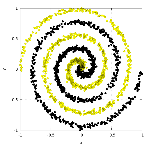
Now let’s try to use the implementation above to train a fully connected neural network for a classification task. For this we use two popular synthetic datasets. The first dataset consists of two noisy intertwined spirals. The second dataset follows the distribution of a checkerboard pattern. Both datasets used for training the model consisted of 20.000 samples. Both validation datasets consisted of 2000 points. The network consisted of three hidden layers with 64 neurons each. The model was trained for 1000 epochs at a learning rate of \(\eta=1e-4\).
Results
The following section shows the results for the validation dataset.
Intertwined Spirals
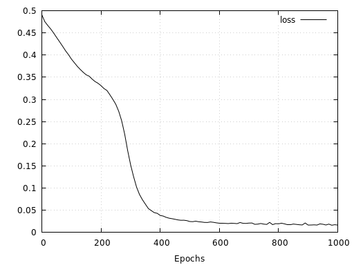
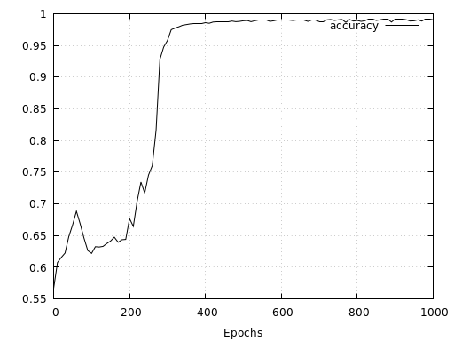
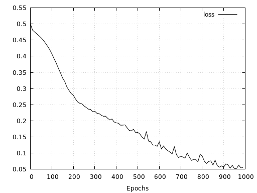
The results for the spirals show that after an initial phase of slow convergence of about 200 epochs, the model converges very quickly and finally reaches a validation accuracy of 99.2%.
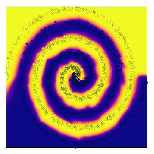
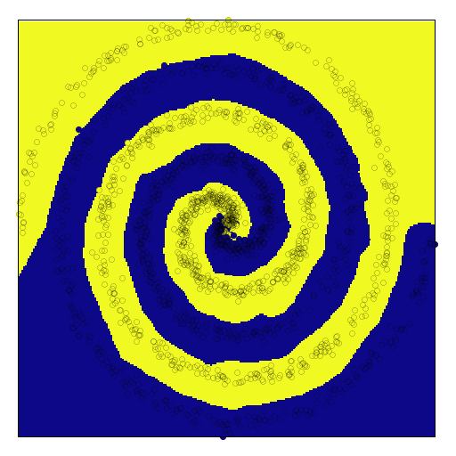
The following two figures show the network’s corresponding continuous and discrete prediction landscape after 1000 epochs of training. Here we see that due to the low noise of both spirals, the network has learned to separate them fairly cleanly.
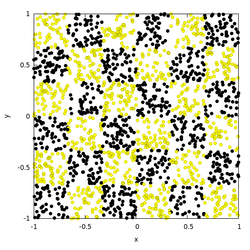
Checkerboard
For the checkerboard, the results are similarly good. The results show a relatively fast convergence of the model reaching 96.8 % validation accuracy after 1000 epochs.
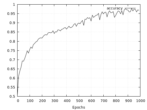
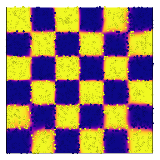
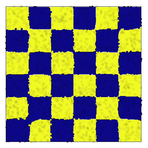
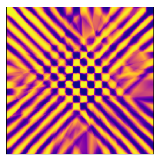
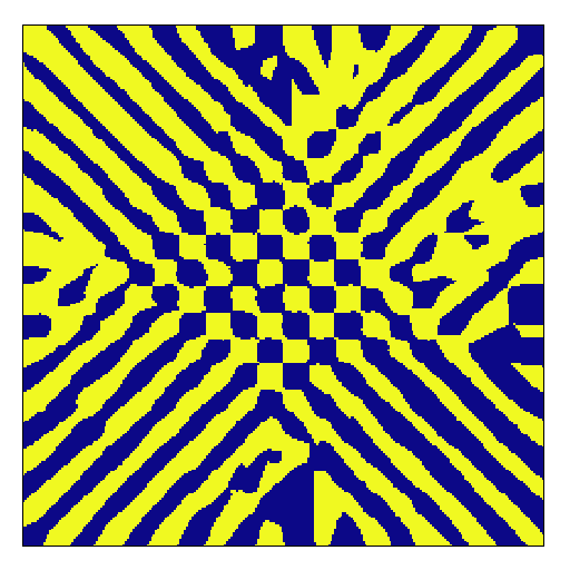
Below we see again the network’s corresponding continuous and discrete prediction landscape for the checkerboard dataset. It is interesting to see how a simple three-layered model of 64 hidden neuron each, can separate the tiles of the checkerboard so cleanly.
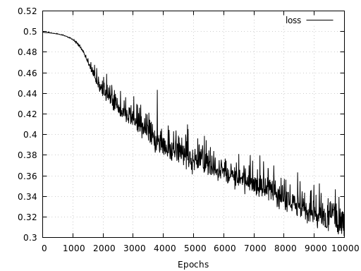
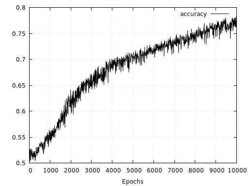
Let’s have a quick look at how the same network performs with a checkerboard pattern consisting of 20 tiles along each axis. Here we see, that even after 10000 epochs and twice the amount of training data, the network is not able to learn the mapping as good as in the simpler case with only 6 tiles along each axis. Both, loss and accuracy show that the network has a much harder time to learn the right representation. At the same time, loss and accuracy also indicate that the network’s capacity has not yet been fully utilized since both measures have not yet converged.
For this pattern we probably need to increase the model’s capacity to allow for a better representation. It is interesting to see that the network has learned to assign only the data points near the origin to the correct classes. For a cleaner visualization of both prediction landscapes below, I removed the validation set data points.
Discussion
This project shows a very basic implementation of a fully connected neural network in C++ with many possibilities for improvement. The results not only show good performance of the network on the selected datasets, but also indicate the correctness of the implementation.
Outlook
The implementation shown in this post should serve as a gentle introduction on how to implement a simple neural networks in C++. The implementation of the fully connected neural network can be extended very easily to deal with an arbitrary number of hidden layers as well as with different activation functions. In addition, the code can be used to try different things. For example, certain layers can be frozen during training without much effort. Also, the implementation can be extended to handle batches. In order to avoid overfitting, regularization methods such as dropout or L2 regularization can be added easily. Last but not least, to speed up the computation you can try to parallelize the multiplication of matrices and vectors so that the program uses more than one core.
You find the code for this project here.