Layer-wise Relevance Propagation with Tensorflow
TL;DR: This post presents a basic implementation of the Layer-wise Relevance Propagation (LRP) algorithm in Tensorflow 2 using the $z^+$-rule.
Introduction
This post presents a simple implementation of the Layer-wise Relevance Propagation (LRP) algorithm in Tensorflow 2 for the VGG16 and VGG19 networks that were pre-trained on the ImageNet dataset. For more information regarding LRP see also here and here.
LRP allows us to better understand the network’s reasoning capabilities by highlighting features that were most relevant for the network’s classification decision. This can enable us, for example, to find flaws in our models more quickly.
Method
Layer-wise relevance propagation allows assigning relevance scores to the network’s activations by defining rules that describe how relevant scores are being computed and distributed. This allows to distinguish between important and less relevant neurons.
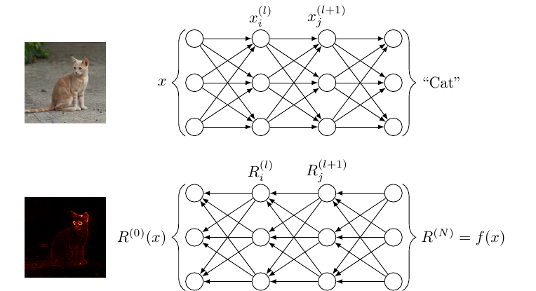
The process of assigning relevance scores to activations starts at the network’s output layer where the activations are used as the initial relevance scores and ends at the input layer where relevance scores are assigned to the input image’s pixels. This process creates a relevance map or heatmap that allows to understand the networks’ classification decision. This process is illustrated in the following figure.
There are several relevance propagation rules. This implementation uses the $z^+$-rule to compute relevance scores and is defined as follows
\begin{equation} \label{eq:zplus} R_i^{(l)} = \sum_j \frac{x_i w_{ij}^+}{\sum_{i’} x_{i’} w_{i’j}^+} R_j^{(l+1)} \end{equation}
Equation \eqref{eq:zplus} describes relevance distribution in fully connected layers. Here, $R_i^{(l)}$ and $R_j^{(l+1)}$ represent the relevance scores of neuron $i$ and $j$ in layers $(l)$ and $(l+1)$, respectively. $x_i$ represents the $i$th neuron’s activation. $w_{ij}^+$ stands for the positive weights connecting the neurons $i$ and $j$ of layers $(l)$ and $(l+1)$.
The first relevance scores correspond to the softmax activations of the network’s output layer. Thus, for a network $f$ consisting of $N$ layers, we can set $R^{(N)} = f(x)$.
From Equation \eqref{eq:zplus} it can also be seen that
\begin{equation} \label{eq:conservation} \sum_m R_m^{(0)} = \dots = \sum_i R_i^{(l)} = \sum_j R_j^{(l+1)} = \dots = \sum_n R_n^{(N)} \end{equation}
which shows that the information of the relevance signal is conserved. This allows us to test the implementation as the sum of all relevance scores per layer should remain 1 for a network that uses the softmax activation function at the output layer.
It is important to note that the relevance scores at the input layer, $R^{(0)}$, must not depend on the image’s pixel values denoted by $x_m$. This would otherwise lead to a biased feature relevance map. For the last computation of relevance scores we therefore set the activations $x_m$ and thus the pixel values to 1. This leads to the $z^+$-rule for the input layer
\begin{equation} \label{eq:zplusinput} R_i^{(l)} = \sum_j \frac{w_{ij}^+}{\sum_{i’} w_{i’j}^+} R_j^{(l+1)} \end{equation}
Implementation
Depending on the information processing operation within the VGG network, relevance information sent back needs to be processed differently. The VGG network consists basically of four different layers: convolutional, pooling, flattening, and fully connected layers. In the subsequent subsections, I will use x, w, and r for the activations, weights, and relevance scores, respectively.
Convolution
Let’s start with the convolutional operations. Here we use the same strides and padding as during the forward pass. We also make sure that the activations are set to one if we reached the input layer. This ensures that the image’s pixel values are not used to compute the relevance scores for the input. Otherwise, we would end up with a biased result. The remaining part corresponds to the $z^+$-rule. In contrast to the information processing in fully connected layers, convolutional operations on feature maps oftentimes overlap depending on the stride. It is therefore necessary to sum up the relevance scores of the feature map activations.
def relprop_conv(self, x, w, r, name, strides=(1, 1, 1, 1), padding='SAME'):
    if name == 'block1_conv1':
        x = tf.ones_like(x)
    w_pos = tf.maximum(w, 0.0)
    z = tf.nn.conv2d(x, w_pos, strides, padding) + self.epsilon
    s = r / z
    c = tf.compat.v1.nn.conv2d_backprop_input(tf.shape(x), w_pos, s, strides, padding)
    return c * x
Pooling
There are two different approaches to send back relevance scores through pooling layers. Either the relevance scores are assigned proportionally based on the neurons’ activation strength or the winner takes it all principle is chosen, in which the highest activation is assigned the entire relevance. In general, max pooling leads to crisper relevance maps by assigning high relevance scores to fewer input features.
def relprop_pool(self, x, r, ksize=(1, 2, 2, 1), strides=(1, 2, 2, 1), padding='SAME'):
    if self.pooling_type == 'avg':
        z = tf.nn.avg_pool(x, ksize, strides, padding) + self.epsilon
        s = r / z
        c = gen_nn_ops.avg_pool_grad(tf.shape(x), s, ksize, strides, padding)
    elif self.pooling_type == 'max':
        z = tf.nn.max_pool(x, ksize, strides, padding) + self.epsilon
        s = r / z
        c = gen_nn_ops.max_pool_grad_v2(x, z, s, ksize, strides, padding)
    else:
        raise Exception('Error: no such unpooling operation.')
    return c * x
Flattening
The flattening operation connects the convolutional part with the fully connected part of the network. Since this operation consists only of reshaping the last feature maps, the backward pass also only consists of reshaping the relevance scores back from a vector representation into the form of feature maps.
def relprop_flatten(self, x, r):
    return tf.reshape(r, tf.shape(x))
Fully connected layers
In the fully connected part of the VGG network, the computation of relevance scores follows directly Equation \eqref{eq:zplus}. The implementation is relatively simple compared to convolutional layers. Namely, there are no shared weights and also no overlapping areas in information processing during the feedforward pass.
def relprop_dense(self, x, w, r):
    w_pos = tf.maximum(w, 0.0)
    z = tf.matmul(x, w_pos) + self.epsilon
    s = r / z
    c = tf.matmul(s, tf.transpose(w_pos))
    return c * x
Experiments
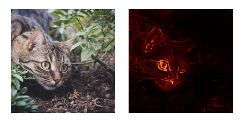
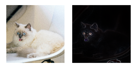
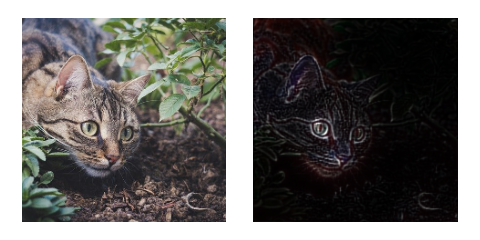
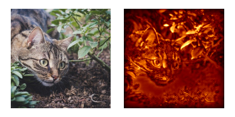
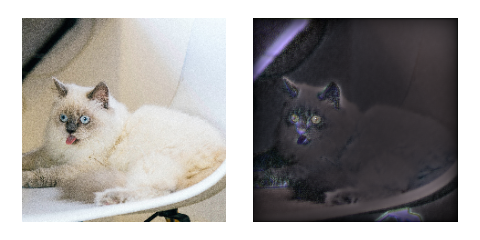
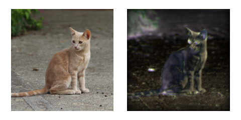
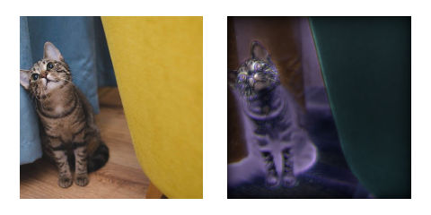
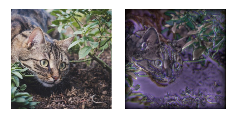
For the experiment, I used several images that I found on the internet with classes that are part of the ImageNet dataset. Since relevance scores are assigned to every pixel, there are two ways of visualizing the resulting relevance map: either pooling the relevance scores along the channel dimension to end up with a kind of grayscale image or by using all three channels resulting in RGB relevance maps.
To further check the plausibility of the results, we can compare the results of a pre-trained VGG network with a randomly initialized network. Relevance scores for randomly initialized networks should assign relevance scores also randomly resulting in a uniform distribution of relevance scores across the input image.
Results
Pre-trained Model
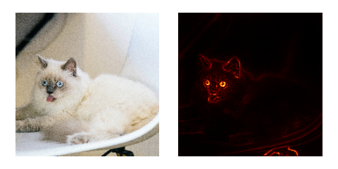
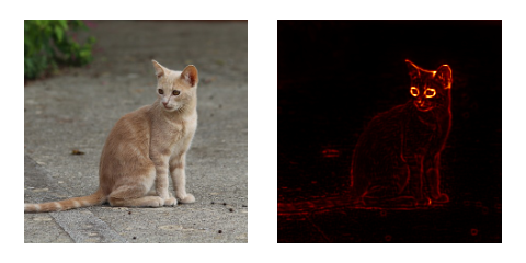
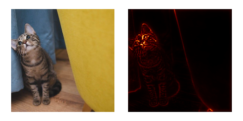
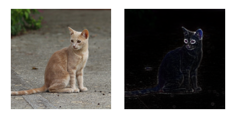
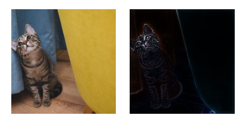
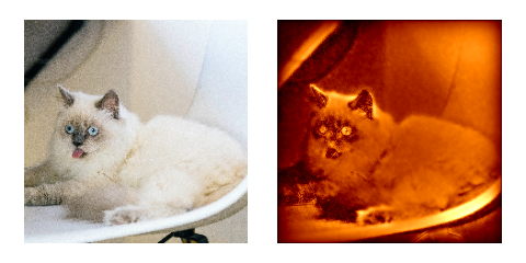
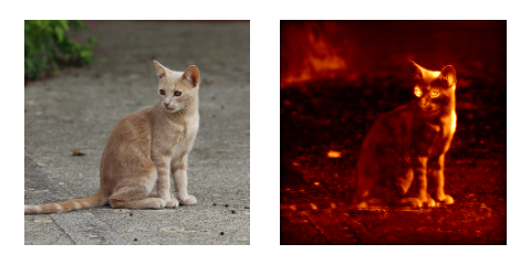
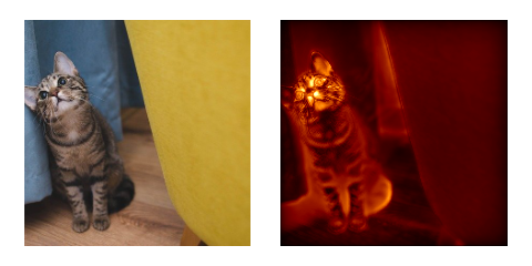
Looking at the computed relevance maps, it turns out that the network’s classification decision is based mainly on features located at the cats’ head. Especially the cats’ eyes seem to be of high importance to the network’s decision. It is interesting to see, that image regions with high contrasts are not subject of high relevance scores, indicating, that the network has learned to distinguish important from unimportant features.
Results for single channel relevance maps.
Results for RGB relevance maps.
Randomly Initialized Model
Relevance maps generated with a randomly initialized VGG16 network show that there are no specific features that the network has learned to associate with the corresponding class. In contrast to the pre-trained model, here the relevance scores are distributed very equally over the entire image.
Results for single channel relevance maps with random weights.
Results for RGB relevance maps with random weights.
Discussion
The qualitative results seem to be plausible since relevance scores are particularly present in those regions of the image that we humans would also associate with the class. It is also interesting to see that few relevance scores were assigned to areas in the image that have little or nothing to do with the class itself. If relevance maps are generated with randomly initialized weights, the assignment of relevance scores is fairly random.
As stated in a paper by Samek et al. the entropy of a relevance score heatmap could also be used as a proxy for its quality or explainability. The idea is, that the entropy, defined as $H = -\sum_m R_m \log (R_m)$, is high if relevance is assigned more randomly across the image domain and low if relevance scores are more concentrated, indicating that the network is familiar with an object and has assigned most relevance scores to it. However, apart from the fact that this approach is not invariant with respect to the object size in the image, entropy is also lower if relevance scores are more concentrated, which does not necessarily mean that the network is familiar with the object or that the quality of a relevance map is high. This is especially true for images containing objects with strong local contrasts.
Outlook
This basic implementation of layer-wise relevance propagation is a good starting point for many possible extensions and applications. For example, new rules for the distribution of relevance scores can be added. Furthermore, one can try to transfer the implementation to more modern network architectures like ResNets or DenseNets.
With a fast graphics card, it is also possible to perform relevance propagation in real time. The following video shows the result of a short test.
It is interesting to note that relevance scores in the background, especially at the door, disappear entirely when the notebook enters the image, which is then assigned a lot of relevance. The network basically indicates that it has recognized something it is familiar with. This is to be expected since the VGG16 network has also been trained to classify notebooks. Here you can find the code for real time relevance propagation.
You find the code for this project here.