NeuralGrid: A Grid-based Neural Network
TL;DR: Grid-based neural network architectures allow neurons to form arbitrary signal processing structures during training.
Introduction
This post presents a grid-based neural network architecture which I will call NeuralGrid. Neural grids are designed to allow artificial neurons to automatically form arbitrary interconnections during the training process, thereby forming a previously undefined network structure. Compared to conventional feedforward network architectures, this approach allows the grid component of the network to be more malleable. The following figure shows the basic structure of a NeuralGrid.
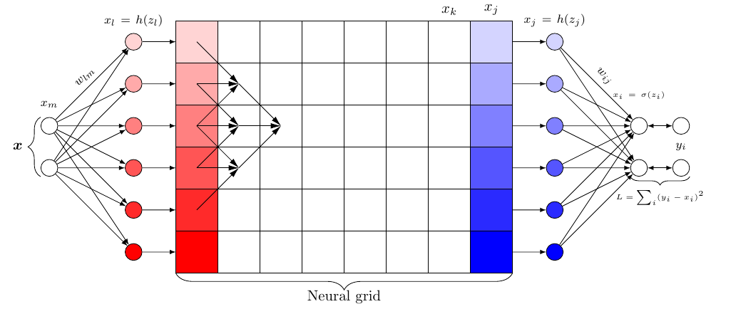 Figure 1: Basic idea of a grid-based neural network architecture.
The image above shows the basic idea behind a grid-based neural network architecture. In a first step, an input $x$ is mapped to the grid’s input dimension where the representation is then processed from left to right using a simple local mapping between adjacent grid layers. The signal at the grid’s output is mapped to the network’s output using again a fully connected layer.
The goal of this project is not to set a new SOTA for some dataset, but rather to investigate qualitatively the emerging patterns within the neural grid and how well the network performs.
Method
The architecture of a two-dimensional grid-based neural network consists of three parts: The mapping from the input neurons $x_m$ to the grid’s first layer, the mapping inside the grid, and finally the mapping from the last grid layer to the network’s output. In case of a three-dimensional grid, the mapping to the grid’s input using a fully connected layer can be skipped as images can be processed directly without converting them first to a vector.
Information Processing Outside the Grid
The network’s information processing consists of two different components. The first type of operation, from the network’s input to the grid’s input, and from the grid’s output to the network’s output consists of a standard vector-matrix multiplication represented by fully connected layers. The information processing of a single neuron outside the grid, i.e. before and after the grid, can be described as an affine linear transformation $z$ that is followed by some nonlinear mapping represented by $h$.
From network’s input to grid’s input:
\begin{equation} \label{eq:preactivation_in} z_l = \sum_{m} w_{lm} x_m + b_l \end{equation}
\begin{equation} \label{eq:activation_in} x_m = h(z_l) \end{equation}
From grid’s output to network’s output:
\begin{equation} \label{eq:preactivation_out} z_i = \sum_{j} w_{ij} x_j + b_i \end{equation}
\begin{equation} \label{eq:activation_out} x_i = h(z_i) \end{equation}
Information Processing Inside the Grid
Things look a bit different for the mapping inside the grid. Here, the mapping is described as follows:
\begin{equation} \label{eq:zgrid} z_p = \sum_{q \subset \Omega_p} w_{q} x_{q} + b_p \end{equation}
\begin{equation} \label{eq:xgrid} x_p = h(z_p) \end{equation}
In Equation \eqref{eq:zgrid}, $\Omega_p$ represents the receptive field over which the weighted sum is calculated. This is shown for the case of a two-dimensional grid in Figure 1 with a receptive field size (i.e. kernel size) of 3 and stride 1. As Figure 1 shows, the weighted sum is computed over three grid cells each. For a three-dimensional grid, the receptive field would be of size $k \times k$. It is also interesting to note, that due to the neural grid’s architecture and the associated processing scheme, there are the same number of biases as there are weights.
Weights within the grid are shared by several neurons due to overlapping receptive fields. Thus, as Figure 1 shows, each weight within the grid contributes to three neurons in the consecutive layer. This must also be taken into account in the gradient computation insofar as the error signals for the respective weights must be accumulated. Fortunately, however, PyTorch’s autograd engine takes care of this for us.
Formulating Grid Processes with Unfolding Operations
There is no out-of-box functionality within the PyTorch library that can perform the processes inside the grid as described above. One possibility would be to create the individual grid cells as a tensor and iterate over the grid with two for-loops. However, this would be incredibly slow (see comparison further below). Luckily, the mapping within the grid can also be represented as a special kind of vector-matrix multiplication, where the matrix is a sparse matrix with shared weights. This allows us to use PyTorch’s blazingly fast unfolding operations which results in a massive speedup compared to a simple loop-based implementation.
The following examples show how the mapping between two consecutive grid layers are formulated using the unfolding operation for the case of a two- and three-dimensional grid.
Unfolding Layers in a Two-Dimensional Neural Grid
For a neural grid layer consisting of activations $\boldsymbol{x}$ and weights $\boldsymbol{w}$ each consisting of five elements, a kernel size of $k=3$, and stride 1, Equation \eqref{eq:zgrid} can be written as
\[\label{eq:2dNeuralGridZ} \boldsymbol{z} = \boldsymbol{w} * \boldsymbol{x} + \boldsymbol{b} = \begin{pmatrix} w_{1}\\ w_{2}\\ w_{3}\\ w_{4}\\ w_{5} \end{pmatrix} * \begin{pmatrix} x_{1}\\ x_{2}\\ x_{3}\\ x_{4}\\ x_{5} \end{pmatrix} + \begin{pmatrix} b_{1}\\ b_{2}\\ b_{3}\\ b_{4}\\ b_{5} \end{pmatrix}\]Here, the symbol $*$ indicates that we perform a local mapping between adjacent layers with a certain kernel size $k$ and shared weights. Now we could rewrite Equation \eqref{eq:2dNeuralGridZ} as follows:
\[\label{eq:sparseWeightMatrix} \boldsymbol{z} = \begin{pmatrix} w_{1} & w_{2} & 0 & 0 & 0\\ w_{1} & w_{2} & w_{3} & 0 & 0\\ 0 & w_{2} & w_{3} & w_{4} & 0\\ 0 & 0 & w_{3} & w_{4} & w_{5}\\ 0 & 0 & 0 & w_{4} & w_{5} \end{pmatrix} \cdot \begin{pmatrix} x_{1}\\ x_{2}\\ x_{3}\\ x_{4}\\ x_{5} \end{pmatrix} + \begin{pmatrix} b_{1}\\ b_{2}\\ b_{3}\\ b_{4}\\ b_{5} \end{pmatrix}\]In Equation \eqref{eq:sparseWeightMatrix} we see that all weights, except for the weights at the grid’s upper and lower end, are involved in three operations, meaning that these weights are shared across several neurons.
From the sparse weight matrix in Equation \eqref{eq:sparseWeightMatrix} it can be read directly that during the backpropagation step, these weights receive three error signals that are used to compute the final gradient. These final gradients can be obtained by summing along the vertical axis of the weight’s matrix corresponding gradient matrix.
However, in terms of memory usage and computational efficiency, Equation \eqref{eq:sparseWeightMatrix} is not very elegant and can be reformulated into a more compact representation
\[\label{eq:unfoldedFormulation} \boldsymbol{z} = \begin{pmatrix} \begin{pmatrix} 0 & w_{1} & w_{2}\\ w_{1} & w_{2} & w_{3}\\ w_{2} & w_{3} & w_{4}\\ w_{3} & w_{4} & w_{5}\\ w_{4} & w_{5} & 0 \end{pmatrix} \odot \begin{pmatrix} 0 & x_{1} & x_{2}\\ x_{1} & x_{2} & x_{3}\\ x_{2} & x_{3} & x_{4}\\ x_{3} & x_{4} & x_{5}\\ x_{4} & x_{5} & 0 \end{pmatrix} \end{pmatrix} \cdot \begin{pmatrix} 1\\ 1\\ 1 \end{pmatrix} + \begin{pmatrix} b_{1}\\ b_{2}\\ b_{3}\\ b_{4}\\ b_{5} \end{pmatrix}\]where $\odot$ represents the element-wise product of weights and activations. The zeros in both the weight and activation matrix, come from same zero padding the vectors in Equation \eqref{eq:2dNeuralGridZ} to ensure that the input layer size is equal to the output layer size. The weight’s and activation’s representation as shown in Equation \eqref{eq:unfoldedFormulation} can be generated from the vector representation in Equation \eqref{eq:2dNeuralGridZ} using PyTorch’s unfold() operation.
At first glance, Equation \eqref{eq:unfoldedFormulation} does not necessarily look more compact. However, this formulation scales with $\mathcal{O}(k \cdot n)$ and is therefore computationally more efficient compared to the first formulation in Equation \eqref{eq:sparseWeightMatrix} that scales with $\mathcal{O}(n^2)$. This is true as long as the kernel size is smaller than the grid’s layer size, which is normally the case.
Unfolding Layers in a Three-Dimensional Neural Grid
We can apply the same logic to the tow-dimensional layers of a three-dimensional neural grid as in the last section. In this case, however, things look a bit trickier. Unlike in the case of standard 2D convolutions as they are implemented in popular machine learning libraries, weights are not shared accross the input (i.e. feature map). Thus, for an image with dimensions $H \times W$ there is the same number of weights per layer as there are pixels. For an input image of size $3 \times 3$, kernel size $k=(3,3)$, and same padding with zeros, the preactivation is computed as follows
\[\label{eq:z3d} \boldsymbol{z} = \boldsymbol{w} * \boldsymbol{x} + \boldsymbol{b} = \begin{pmatrix} w_{1} & w_{2} & w_{3} \\ w_{4} & w_{5} & w_{6} \\ w_{7} & w_{8} & w_{9} \end{pmatrix} * \begin{pmatrix} x_{1} & x_{2} & x_{3} \\ x_{4} & x_{5} & x_{6} \\ x_{7} & x_{8} & x_{9} \end{pmatrix} + \begin{pmatrix} b_{1} & b_{2} & b_{3}\\ b_{4} & b_{5} & b_{6}\\ b_{7} & b_{8} & b_{9} \end{pmatrix}\]Again, we can rewrite the computation of the preactivation in Equation \eqref{eq:z3d} with unfolding operations as follows:
\[\Tiny \label{eq:z3dunfolded} \boldsymbol{z} = \begin{pmatrix} \begin{pmatrix} \begin{pmatrix} 0 & 0 & 0 & 0 & w_{1} & w_{2} & 0 & w_{4} & w_{5}\\ 0 & 0 & 0 & w_{1} & w_{2} & w_{3} & w_{4} & w_{5} & w_{6}\\ 0 & 0 & 0 & w_{2} & w_{3} & 0 & w_{5} & w_{6} & 0 \\ 0 & w_{1} & w_{2} & 0 & w_{4} & w_{5} & 0 & w_{7} & w_{8}\\ w_{1} & w_{2} & w_{3} & w_{4} & w_{5} & w_{6} & w_{7} & w_{8} & w_{9}\\ w_{2} & w_{3} & 0 & w_{5} & w_{6} & 0 & w_{8} & w_{9} & 0 \\ 0 & w_{4} & w_{5} & 0 & w_{7} & w_{8} & 0 & 0 & 0 \\ w_{4} & w_{5} & w_{6} & w_{7} & w_{8} & w_{9} & 0 & 0 & 0 \\ w_{5} & w_{6} & 0 & w_{8} & w_{9} & 0 & 0 & 0 & 0 \end{pmatrix} \odot \begin{pmatrix} 0 & 0 & 0 & 0 & x_{1} & x_{2} & 0 & x_{4} & x_{5}\\ 0 & 0 & 0 & x_{1} & x_{2} & x_{3} & x_{4} & x_{5} & x_{6}\\ 0 & 0 & 0 & x_{2} & x_{3} & 0 & x_{5} & x_{6} & 0 \\ 0 & x_{1} & x_{2} & 0 & x_{4} & x_{5} & 0 & x_{7} & x_{8}\\ x_{1} & x_{2} & x_{3} & x_{4} & x_{5} & x_{6} & x_{7} & x_{8} & x_{9}\\ x_{2} & x_{3} & 0 & x_{5} & x_{6} & 0 & x_{8} & x_{9} & 0 \\ 0 & x_{4} & x_{5} & 0 & x_{7} & x_{8} & 0 & 0 & 0 \\ x_{4} & x_{5} & x_{6} & x_{7} & x_{8} & x_{9} & 0 & 0 & 0 \\ x_{5} & x_{6} & 0 & x_{8} & x_{9} & 0 & 0 & 0 & 0 \end{pmatrix} \end{pmatrix} \cdot \begin{pmatrix} 1\\ 1\\ 1\\ 1\\ 1\\ 1\\ 1\\ 1\\ 1 \end{pmatrix} \end{pmatrix}^{H \times W} + \boldsymbol{b}\]Here, $(\cdot)^{H \times W}$ denotes the reshaping of the resulting column vector into a matrix with size $H \times W$. In Equation \eqref{eq:z3dunfolded} we can see that every row in the weight and activation matrices correspond to a single feature in the following layer.
Equation \eqref{eq:z3dunfolded} already indicates that in the case of a three-dimensional neural grid with its two-dimensional layers that unfolding becomes computational expensive really quickly and by that slowing down training significantly. Here it is becoming clear that the unfolding operation as provided by PyTorch’s library is a good tool to describe the mappings between grid layers, but for an efficient solution one would have to write a separate kernel or wait until something more efficient is available.
Implementation
Naive Implementation of a Neural Grid
When I first implemented the idea of a neural grid, I took a very naive approach of iterating through a grid of tensors using two for-loops. Sure, this approach works, but required many hours to train even a single epoch on the Fashion-MNIST dataset. The entire forward() method in the NeuralGrid class was a gigantic bottleneck - especially since the implementation could process only a single sample at a time (i.e. batch size of one). If at all, using the naive implementation below, the neural grid could only crawl at best.
The following snippet of code shows the low-level implementation of a neural grid in PyTorch using two for-loops to iterate over the grid. The full details of the implementation are available in the corresponding Github repository of this project linked at the end of this post.
class NeuralGrid(nn.Module):
    """
    Implements a naive version of a neural grid in PyTorch
    """
    def __init__(self, params):
        super().__init__()
        # ...

    def forward(self, x):
        x = x.reshape(self.grid_height)

        # Assign data to grid
        for i in range(self.grid_height):
            self.a[i + 1][0] = x[i]

        # Feed data through grid
        for j in range(self.grid_width):
            for i in range(self.grid_height):
                z = self.a[i - 1][j] * self.w[i - 1][j] \
                    + self.a[i][j] * self.w[i][j] \
                    + self.a[i + 1][j] * self.w[i + 1][j] \
                    + self.b[i][j]
                self.a[i + 1][j + 1] = self.activation_function(z)

        # Assign grid output to new vector
        x_out = torch.zeros(size=(self.grid_height,))
        for i in range(self.grid_height):
            x_out[i] = self.a[i + 1][-1]

        x_out = x_out.reshape(1, self.grid_height)

        return x_out
Implementation of a Neural Grid using Unfolding
I then wondered how to reformulate the problem on hand to increase computational speed, an realized that the mapping between layers in the grid can be formulated using a special form of vector-matrix multiplication as shown in Equation \eqref{eq:sparseWeightMatrix}. From there, it didn’t take long to come up with writing the whole thing using unfolding operations.
This approach resulted in the following implementation consisting of two classes. The NeuralGrid and the GridLayer class. The GridLayer class creates the trainable parameters for each layer and defines the corresponding mapping between adjacent grid layers. In contrast to the naive approach above, in GridLayer we reformulate the inner for-loop by combining unfolding with an element-wise product followed by a sum along the resulting matrix’s rows.
class GridLayer(nn.Module):
    """Class implements layer of a neural grid
    """
    def __init__(self, params):
        super().__init__()

        grid_height = params["grid_2d"]["height"]

        self.kernel_size = 3  # kernels must be of size 2n+1 where n>0
        self.stride = 1
        self.padding = int(0.5 * (self.kernel_size - 1))

        # Trainable parameters
        weight = xavier_init(size=(grid_height,), fan_in=self.kernel_size, fan_out=self.kernel_size)
        weight = F.pad(input=weight, pad=[self.padding, self.padding], mode="constant", value=0.0)
        self.weight = nn.Parameter(weight, requires_grad=True)
        self.bias = nn.Parameter(torch.zeros(size=(grid_height,)), requires_grad=True)

        self.activation_function = torch.sin

    def forward(self, x_in):
        # Same padding to ensure that input size equals output size
        x = F.pad(input=x_in, pad=[self.padding, self.padding], mode="constant", value=0.0)

        # Unfold activations and weights for grid operations
        x = x.unfold(dimension=1, size=self.kernel_size, step=self.stride)
        w = self.weight.unfold(dimension=0, size=self.kernel_size, step=self.stride)

        # Compute pre-activation
        x = (w * x).sum(dim=-1) + self.bias

        # Compute activations
        x = self.activation_function(x)

        return x
In the NeuralGrid class, we simply iterate over each layers of the grid mapping the features from the grid’s input to its output.
class NeuralGrid(nn.Module):
    """ Implements a neural grid
    """

    def __init__(self, params):
        super().__init__()

        grid_width = params["grid_2d"]["width"]

        # Add grid layers to a list
        self.grid_layers = nn.ModuleList()
        for _ in range(grid_width):
            self.grid_layers.append(GridLayer(params))

    def forward(self, x):
        for grid_layer in self.grid_layers:
            x = grid_layer(x)
        return x
Comparison of Implementations
I wondered how both implementations above would compare in terms of their computational performance and tested how long it would take each approach to do a single epoch. So let’s look at some numbers how the implementations perform using the Fashion-MNIST dataset and a grid size of $128 \times 128$. The structure of the entire network is therefore $784 \times [128 \times 128] \times 10$.
The following table shows the training time in seconds for a single epoch on the Fashion-MNIST dataset for different batch sizes and accelerators.
| Implementation | Accelerator | Batch size | Time per epoch | Speedup |
|---|---|---|---|---|
| Double loop | CPU | $1$ | $52427 \pm 607$ s (~14 h) | $1$ |
| Unfold | CPU | $1$ | $1503 \pm 288$ s | $34$ |
| Unfold | CPU | $16$ | $404 \pm 59$ s | $129$ |
| Unfold | CPU | $32$ | $329 \pm 33$ s | $159$ |
| Unfold | CPU | $64$ | $257 \pm 4$ s | $203$ |
| Unfold | GPU | $64$ | $21 \pm 1$ s | $2469$ |
| Unfold | GPU | $256$ | $5.41 \pm 0.17$ s | $9687$ |
As the table shows, using unfolding operations in combination with a GPU an increase of processing speed by about four orders of magnitude were possible.
Experiments
The main focus of the experiments was to gather qualitative insights on how grid-based neural networks behave in a supervised classification task. For this reason, a grid-based model with a grid size of $64 \times 64$ cells was trained on the Fashion-MNIST dataset by optimising the multinomial logistic regression objective (softmax function) using the Adam optimization algorithm. The batch size during training was set to $256$. The learning rate was initially set to $1 \times 10^{-4}$, and then decreased by a factor of $10$ every $100$ epochs. In total, the learning was stopped after $300$ epochs. The grid’s weights were initialized using the Xavier initialization scheme. The biases were initialized with zero. In order to force the grid to learn better representations, a linear mapping was used from the network’s input to the grid’s input. The sine function was chosen as the activation function within the grid, since it allowed for significantly deeper grids.
Results and Discussion
The grid-based neural network achieved an classification accuracy of $86.9 \%$ on the Fashion-MNIST dataset. The following two figures show some qualitative results of the neural grid’s activation pattern at the start and at the end of training for the ten classes of the Fashion-MNIST dataset. For each activation pattern, the activations of the first $64$ samples of each class were averaged.
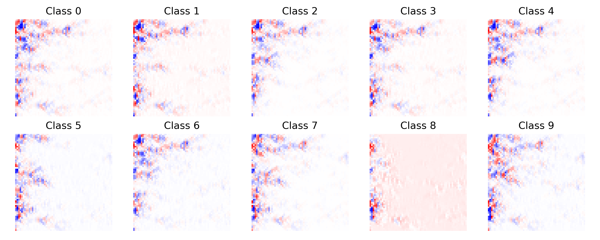 Figure 2: Neural grid activation patterns at the start of training.
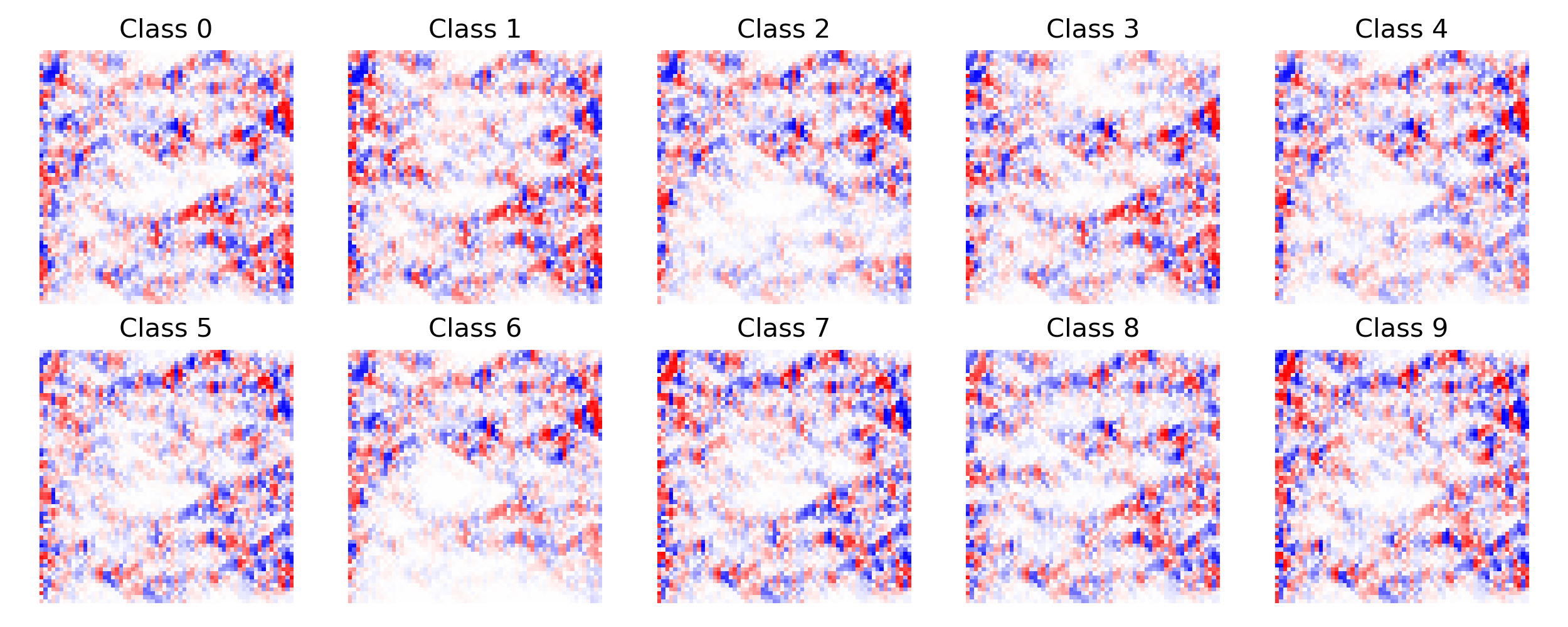 Figure 3: Neural grid activation patterns at the end of training.
It is interesting to see that the activation pattern before the training is not very pronounced. At the end of training, however, very clear structures have emerged. It is also noticeable, that depending on the class, the signal uses mostly different paths through the neural grid and by that is processed differently. However, it can also be seen that some paths are active in all activation patterns regardless the class. This could be an indication that the grid has not yet been sufficiently trained.
In general, training larger neural grids is more difficult due to common problems such as vanishing or exploding gradients. However, with the sine activation function it was possible to train larger grids with more than $128$ layers, which is quite impressive for such a network without residual connections.
Conclusion
This blog post introduced a grid-based neural network architecture. Neural grids can be understood as a discretized signal processing network, where information are processed in a feedforward manner. The neural grid’s placticity also allows to form arbitrary network structures within the grid. The qualitative results have shown, that such pathways for the routing of signals emerge in the grid during training automatically.
@misc{Fischer2021gnn,
  title={NeuralGrid: A Grid-based Neural Network},
  author={Fischer, Kai},
  howpublished={\url{https://kaifishr.github.io/2021/04/06/neural-grid.html}},
  year={2021}
}
You find the code for this project here.