Gradient-based Weight Extrapolation
TL;DR: Information stored in previously computed gradients can be used for additional weight extrapolation steps during training using the Taylor series expansion combined with backward differentiation.
Introduction
Improving gradient based optimization is an important aspect as it also allows large neural networks and other machine learning models to learn not only faster but also better representations of the data provided. In this post I want to explore how information stored in past gradients computed during the optimization process can be exploited to extrapolate the model’s trainable parameters to predict a new set of weights and biases between two gradient descent steps. The following figure illustrates the idea of extrapolating model parameters.
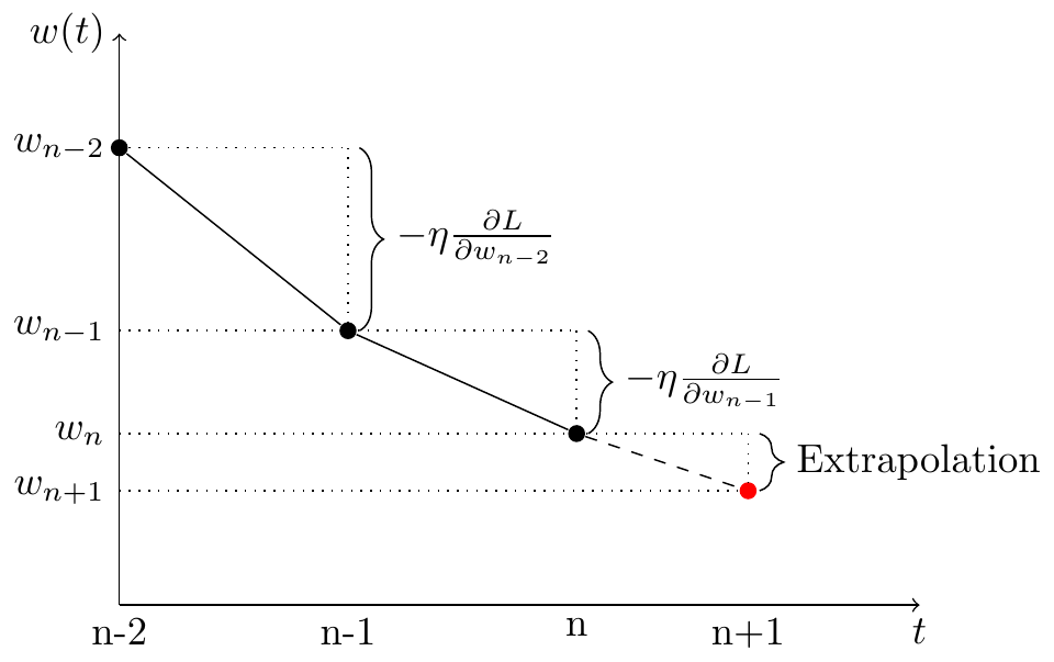
Figure 1: Schematic drawing of how past gradient information can be used to predict a new set of model parameters at $n+1$.
Figure 1 shows the basic idea how information about previously computed gradients can be used to perform intermediate weight extrapolation steps. For an extrapolation step of second-order, the current and previous gradients are needed to compute a new set of parameters. The illustration shows that this is equivalent to using the information of the last three parameter states.
Method
The method consists of using the Taylor series expansion of the unknown function $w(t)$ describing the model parameters’ behavior in parameter space, to derive an expression for an update rule that represents an extrapolation step. Here, $w(t)$ describes a single trainable parameter’s trajectory as a function of time. This extrapolation step, executed between two gradient descent optimization steps, allows to determine a new set of parameters based on past gradient information.
The Taylor series of a function $w(t)$ at point $t_{0}$ is the power series
\[w(t) = \sum_{k=0}^{\infty} \frac{w^{(k)}(t)}{k!}\bigg\rvert_{t=t_{0}}(t-t_{0})^k\]Here, we are going to use the third-order Taylor series expansion to derive the formula describing an extrapolation step:
\[\begin{equation} \begin{aligned} \label{eq:taylorExpansion} w(t) = w(t)\bigg\rvert_{t=t_{0}} &+ w'(t)\bigg\rvert_{t=t_{0}}(t-t_{0}) \\ &+ \frac{1}{2}w''(t)\bigg\rvert_{t=t_{0}}(t-t_{0})^2\\ &+ \frac{1}{6}w'''(t)(t-t_{0})^3\bigg\rvert_{t=t_{0}} + \mathcal{O}(t^4) \end{aligned} \end{equation}\]For the extrapolation we are trying to guess $w(t)$ at $t=t_{0}+\Delta t$. The step size is thus just $\Delta t = t-t_{0}$. Inserting both expressions above leads to
\[w(t_{0}+\Delta t) = w(t_{0}) + w'(t_{0})\Delta t + \frac{1}{2}w''(t_{0})\Delta t^2 + \frac{1}{6}w'''(t_{0})\Delta t^3 + \mathcal{O}(t^4)\]To make thinks look a bit friendlier, I’ll use the following notation $w(t_{0}) = w_{n}$ and $w(t_{0}+\Delta t) = w_{n+1}$, where the index $n$ represents the current optimization step. This leads us to the following expression:
\[\label{eq:thirdOrderExtrapolation} w_{n+1} = w_{n} + w'_{n}\Delta t + \frac{1}{2}w''_{n}\Delta t^2 + \frac{1}{6}w'''_{n}\Delta t^3 + \mathcal{O}(\Delta t^4)\]Equation \eqref{eq:thirdOrderExtrapolation} tells us, that for performing an extrapolation step, we need higher-order derivatives of $w_{n}$. Now we are left with finding good approximations for the derivatives of $w_{n}$ about $t_{0}$.
There are several methods to approximate these derivatives. I’ll start with a fairly straightforward approach where I use the finite backward difference method to approximate higher-order derivatives. After that, I’ll derive higher-order derivatives using the backward differentiation formula.
Finite Backward Differences
The derivative of $w(t)$ at point $t$ is defined as the limit when we let $h$ go to zero
\[\label{eq:definitionDerivative} w'(t) = \lim_{h \rightarrow 0} \frac{w(t)-w(t-h)}{h},\]also known as the differences quotient. To compute the derivatives in Equation \eqref{eq:thirdOrderExtrapolation}, we can use finite differences. A finite difference is often used to approximate derivatives, typically in numerical differentiation. Here, we use the backward difference since we only have the parameters’ previous states available to work with, meaning the function values at $t$ and $t-h$:
\[\label{eq:backwardDifference} \nabla_{h}[w](t) = w(t) - w(t-h)\]The finite difference above divided by $h$ results in a difference quotient. More specifically, if $h$ has a fixed non-zero value instead of approaching zero, then the right-hand side of the Equation \eqref{eq:definitionDerivative} would be written as follows
\[\label{eq:firstOrderBackward} w'(t) = \frac{\nabla^1_{h}[w](t)}{h} = \frac{w(t)-w(t-h)}{h} + \mathcal{O}(h).\]which is already the first-order backward difference quotient. To derive the second-order backward difference we recursively insert the first-order backward difference into its own definition which leads to
\[\begin{equation} \begin{aligned} \label{eq:secondOrderBackward} w''(t) &= \frac{\nabla^2_{h}[w](t)}{h^2} + \mathcal{O}(h)\\ &= \frac{w'(t)-w'(t-h)}{h} + \mathcal{O}(h)\\ &= \frac{\frac{w(t)-w(t-h)}{h}-\frac{w(t-h)-w(t-2h)}{h}}{h} + \mathcal{O}(h)\\ &= \frac{w(t)-2w(t-h)+w(t-2h)}{h^2} + \mathcal{O}(h). \end{aligned} \end{equation}\]For the third-order backward difference we get
\[\begin{equation} \begin{aligned} \label{eq:thirdOrderBackward} w'''(t) &= \frac{\nabla^3_{h}[w](t)}{h^3} + \mathcal{O}(h)\\ &= \frac{w(t)-3w(t-h)+3w(t-2h)-w(t-3h)}{h^3} + \mathcal{O}(h). \end{aligned} \end{equation}\]As an aside, by examining the pattern for the expressions above more closely, one sees that a general finite backward difference formula exists:
\[\nabla_{h}^{n}[w](t) = \sum_{i=0}^n (-1)^i {n \choose i} w(t-ih).\]What remains now, is to formulate the derivatives’ approximations in terms of information available to us during training. To do that, I’ll use the most basic gradient update rule
\[\label{eq:updateRule} w_{n} = w_{n-1} - \eta \frac{\partial L}{\partial w_{n-1}}.\]where $\frac{\partial L}{\partial w_{n-1}}$ represents the change of the loss represented by $L$ with respect to model weight $w$ at optimization step $n-1$. Using Equation \eqref{eq:updateRule} we can express the approximations of the derivatives using gradients computed during the optimization process. I’m going to use the notation $w_{n-1} = w(t-h)$ and $\partial_{w_{n-1}} L = \frac{\partial L}{\partial w_{n-1}}$ to present the expressions in a more tidy way. Now, we omit higher-order terms and get the following expressions for the first, second, and third derivative:
\[\begin{equation} \begin{aligned} \label{eq:firstOrderBackward2} w'_{n} &= \frac{w_{n}-w_{n-1}}{h}\\ &= -\frac{\eta}{h}\partial_{w_{n-1}} L \end{aligned} \end{equation}\] \[\begin{equation} \begin{aligned} \label{eq:secondOrderBackward2} w''_{n} &= \frac{(w_{n}-w_{n-1})-(w_{n-1}-w_{n-2})}{h^2}\\ &= -\frac{\eta}{h^2}(\partial_{w_{n-1}} L - \partial_{w_{n-2}} L) \end{aligned} \end{equation}\] \[\begin{equation} \begin{aligned} \label{eq:thirdOrderBackward2} w'''_{n} &= \frac{(w_{n}-w_{n-1}) - 2(w_{n-1}-w_{n-2}) + (w_{n-2}-w_{n-3})}{h^3}\\ &= -\frac{\eta}{h^3}(\partial_{w_{n-1}} L - 2\partial_{w_{n-2}} L + \partial_{w_{n-3}} L) \end{aligned} \end{equation}\]Inserting Equation \eqref{eq:firstOrderBackward2}, \eqref{eq:secondOrderBackward2}, and \eqref{eq:thirdOrderBackward2} into Equation \eqref{eq:thirdOrderExtrapolation} yields
\[\begin{equation} \begin{aligned} \label{eq:thirdOrderExtrapolationBackward} w_{n+1} = w_{n} &- \frac{\eta\Delta t}{h} \partial_{w_{n-1}} L \\ &- \frac{\eta\Delta t^2}{2h^2}\left( \partial_{w_{n-1}} L - \partial_{w_{n-2}} L\right) \\ &- \frac{\eta\Delta t^3}{6h^3}\left( \partial_{w_{n-1}} L - 2\partial_{w_{n-2}} L + \partial_{w_{n-3}} L \right) \end{aligned} \end{equation}\]Now, Equation \eqref{eq:thirdOrderExtrapolationBackward} only contains known expressions allowing to perform an extrapolation step starting from $w_{n}$. By looking at the first term of Equation \eqref{eq:thirdOrderExtrapolationBackward}, we see that we recovered the standard gradient descent update rule with step size $\frac{\eta \Delta t}{h}$.
As an aside, for a small but finite $h$ we can approximate the derivative $w’(t)$ by $w’(t) \approx \frac{w_{t}-w_{t-1}}{\eta}$ and thus we have $h \equiv \eta$. This approximation is valid for small learning rates $\eta$. However, using small learning rates during training can take our model ages to converge. On the other hand, relatively large learning rates lead to a poor approximation of \(w(t)'\), \(w(t)''\), and \(w(t)'''\) necessary for the extrapolation to work. So there is a certain trade-off worth considering when we test the proposed method. Aside over.
At this point I would like to emphasize that the formulation above for parameter extrapolation contains higher-order derivatives that deliver good results only for very learning rates $\eta$. For this reason, better approximations for the derivatives of $w(t)$ will be derived in the following section.
Backward Differentiation Formula
In this section I’ll derive a backward differentiation formula (BDF) that allows better approximations for the derivatives of $w(t)$. The approach used is an implicit method for the numerical integration of ordinary differential equations (ODE) of the form
\[\label{eq:ode} \frac{dw(t)}{dt} = f(t, w(t)).\]The method works analogously also for higher derivatives of $w(t)$. As we don’t have a closed form of $w(t)$ we can write the left hand side of Equation \eqref{eq:ode} as a linear combination of values we know $w_{n-1}, w_{n-2}, \cdots$, representing past parameter states, and the values we are searching for $a_{n}, a_{n-1}, \cdots$. We start with approximating the first derivative expressed by
\[\label{eq:odeAnsatz} \frac{dw(t)}{dt}\bigg\rvert_{t=t_{n}} = \sum_{i=0}^{n} a_{n-i} w_{n-i}.\]For the approximation of the first derivative I’m going to use four linear combinations
\[\label{eq:bdfApproximationFirstDerivative} \frac{dw(t)}{dt}\bigg\rvert_{t=t_{n}} = a_{n}w_{n} + a_{n-1}w_{n-1} + a_{n-2}w_{n-2} + a_{n-3}w_{n-3}.\]Now we are going to determine the coefficients $a$ of the linear combinations above by replacing the known values ($w_{n-1}$, $w_{n-2}$, and $w_{n-3}$, i.e., the parameter’s past states) with Taylor expansions about $\tau = t_{n}$. The Taylor expansion of a function $w(t)$ is given by
\[\label{eq:taylorExpansionBDF} w(t) = \sum_{k=0}^{\infty} \frac{w^{(k)}(t)}{k!}\bigg\rvert_{t=\tau}(t-\tau)^k\]To compute an approximation of $w_{n-1}$, we use $t = \tau - h$ or $t - \tau = -h$ in Equation \eqref{eq:taylorExpansionBDF}. To make the notation more readable, we’ll use $\tau = t_{n} = t+h$, $w(t_{n})=w_{n}$, and $w(t_{n}-h)=w_{n-1}$.
\[w_{n-1} = \sum_{k=0}^{\infty} \frac{w^{(k)}(t)}{k!}\bigg\rvert_{t=\tau}(-h)^k\]Expanding the equation above for $w_{n-1}$ yields
\[\begin{equation} \begin{aligned} w_{n-1} = w_{n} - h w_{n}' + \frac{1}{2}h^2w_{n}'' - \frac{1}{6}h^3w_{n}''' + \mathcal{O}(h^4) \end{aligned} \end{equation}\]Now, that we have addressed the case for $t = \tau - h$ to derive $w_{n-1}$, let us consider the case for $t = \tau - 2h$ to derive $w_{n-2}$. By inserting $t - \tau = -2h$ into Equation \eqref{eq:taylorExpansionBDF}, we get the following expression for $w_{n-2}$
\[\begin{equation} \begin{aligned} w_{n-2} &= \sum_{k=0}^{\infty} \frac{w^{(k)}(t)}{k!}\bigg\rvert_{t=\tau}(-2h)^k\\ &= w_{n} - 2hw_{n}' + 2h^2w_{n}'' - \frac{4}{3}h^3w_{n}''' + \mathcal{O}(h^4) \end{aligned} \end{equation}\]Now, only $w_{n-3}$ is missing. Here we proceed analogously. We want an expression for $w(t)$ at $t = \tau - 3h$. Inserting $t - \tau = -3h$ into Equation \eqref{eq:taylorExpansionBDF} yields
\[w_{n-3} = w_{n} - 3hw_{n}' + \frac{9}{2}h^2w_{n}'' - \frac{9}{2}h^3w_{n}''' + \mathcal{O}(h^4)\]Since we want to find the value of $w_{n}$ at time $t_{n}$ that balances the ordinary differential equation in Equation \eqref{eq:ode} we now replace the known values (past states) with our Taylor expansions about $\tau = t_{n}$ in Equation \eqref{eq:bdfApproximationFirstDerivative}. Substituting the Taylor expansions for $w_{n-1}$, $w_{n-2}$, and $w_{n-3}$ into Equation \eqref{eq:bdfApproximationFirstDerivative} results in the following expression
\[\begin{equation} \begin{aligned} w_{n}' & = a_{n} w_{n}\\ & + a_{n-1} (w_{n} - hw'_{n} + \frac{1}{2}h^2w''_{n} - \frac{1}{6}h^3w'''_{n})\\ & + a_{n-2} (w_{n} - 2hw'_{n} + 2h^2w''_{n+1} - \frac{4}{3}h^3w'''_{n})\\ & + a_{n-3} (w_{n} - 3hw'_{n} + \frac{9}{2}h^2w''_{n} - \frac{9}{2}h^3w'''_{n}) + \mathcal{O}(h^4) \end{aligned} \end{equation}\]We can rewrite the expression above and get
\[\begin{equation} \begin{aligned} \label{eq:bdfApproximationTaylor} w_{n}' & = (a_{n} + a_{n-1} + a_{n-2} + a_{n-3}) w_{n}\\ & + (0a_{n} - ha_{n-1} - 2ha_{n-2} - 3ha_{n-3})w'_{n}\\ & + (0a_{n} + \frac{1}{2}h^2a_{n-1} + 2h^2a_{n-2} - \frac{9}{2}h^2a_{n-3})w''_{n}\\ & + (0a_{n} - \frac{1}{6}h^3a_{n-1} - \frac{4}{3}h^3a_{n-2} - \frac{9}{2}h^3a_{n-3})w'''_{n} + \mathcal{O}(h^4) \end{aligned} \end{equation}\]In order to get the best approximation for $w_{n}’$ we search for coefficients $a_{i}$ so that Equation \eqref{eq:bdfApproximationTaylor} is satisfied. We can find the coefficients that satisfy Equation \eqref{eq:bdfApproximationTaylor} by expressing the problem as a square linear system of equations.
\[\begin{equation} \begin{aligned} \label{eq:linearSystemOfEquations} a_{n} + a_{n-1} + a_{n-2} + a_{n-3} = 0\\ 0 - ha_{n-1} - 2ha_{n-2} - 3ha_{n-3} = 1\\ 0 + \frac{1}{2}h^2a_{n-1} + 2h^2a_{n-2} - \frac{9}{2}h^2a_{n-3} = 0\\ 0 - \frac{1}{6}h^3a_{n-1} - \frac{4}{3}h^3a_{n-2} - \frac{9}{2}h^3a_{n-3} = 0 \end{aligned} \end{equation}\]Which can also expressed as
\[\begin{equation} \begin{aligned} \begin{pmatrix} 1 & 1 & 1 & 1 \\ 0 & -h & -2h & -3h \\ 0 & \frac{1}{2}h^2 & 2h^2 & \frac{9}{2}h^2 \\ 0 & -\frac{1}{6}h^3 & -\frac{4}{3}h^3 & -\frac{9}{2}h^3 \end{pmatrix} \cdot \begin{pmatrix} a_{n}\\ a_{n-1}\\ a_{n-2}\\ a_{n-3} \end{pmatrix} = \begin{pmatrix} 0\\ 1\\ 0\\ 0 \end{pmatrix} \end{aligned} \end{equation}\]Solving this system of linear equations results in
\[a_{n} = \frac{11}{6h},\hspace{4mm} a_{n-1} = -\frac{3}{h},\hspace{4mm} a_{n-2} = \frac{3}{2h}, \hspace{4mm} a_{n-3} = -\frac{1}{3h}\]These parameters can now be substituted into Equation \eqref{eq:bdfApproximationFirstDerivative}, leading to an approximation for $w_{n}’$ given the current, $w_{n}$, and previous states $w_{n-1}$, $w_{n-2}$, and $w_{n-3}$. Ignoring higher-order terms we get the following expression
\[\begin{equation} \begin{aligned} \label{eq:bdfFirstOrderDerivative} w_{n}' &= \frac{11}{6h}w_{n} - \frac{3}{h}w_{n-1} + \frac{3}{2h}w_{n-2} - \frac{1}{3h}w_{n-3}\\ &= \frac{1}{h}(\frac{11}{6}w_{n} - 3w_{n-1} + \frac{3}{2}w_{n-2} - \frac{1}{3}w_{n-3}) \end{aligned} \end{equation}\]We can rewrite Equation \eqref{eq:bdfFirstOrderDerivative} using the gradient update rule from Equation \eqref{eq:updateRule} so that we can compute $w_{n}’$ using the gradients computed during the gradient descent optimization:
\[\begin{equation} \begin{aligned} \label{eq:bdfFirstOrderDerivativeGradients} w_{n}' &= \frac{1}{h}(\frac{11}{6}w_{n} - \frac{18}{6}w_{n-1} + \frac{9}{6}w_{n-2} - \frac{2}{6}w_{n-3})\\ &= \frac{1}{6h}(11(w_{n} - w_{n-1}) - 7(w_{n-1}-w_{n-2}) + 2(w_{n-2}-w_{n-3}))\\ &= \frac{1}{6h}(11(-\eta \partial_{w_{n-1}}L) - 7(-\eta \partial_{w_{n-2}}L) + 2(-\eta \partial_{w_{n-3}}L))\\ &= -\frac{\eta}{6h}(11\partial_{w_{n-1}}L - 7\partial_{w_{n-2}}L + 2\partial_{w_{n-3}}L) \end{aligned} \end{equation}\]Now, the expression for $w_{n}’$ can be used directly in an optimizer that holds the current and past to gradients. The derivations for $w_{n}’’$ and $w_{n}’’’$ follow exactly the same pattern. Therefore, I will only roughly sketch these two derivations.
Solving the system of linear equations for $w_{n}’’$ results in
\[a_{n} = \frac{2}{h^2},\hspace{4mm} a_{n-1} = -\frac{5}{h^2},\hspace{4mm} a_{n-2} = \frac{4}{h^2}, \hspace{4mm} a_{n-3} = -\frac{1}{h^2}\]We substitute again these parameters into Equation \eqref{eq:bdfApproximationFirstDerivative}, resulting in an approximation for $w_{n}’’$ given the previous states $w_{n}$, $w_{n-1}$, $w_{n-2}$, and $w_{n-3}$.
\[\begin{equation} \begin{aligned} \label{eq:bdfSecondOrderDerivative} w_{n}'' &= a_{n}w_{n} + a_{n-1}w_{n-1} + a_{n-2}w_{n-2} + a_{n-3}w_{n-3}\\ &= \frac{2}{h^2}w_{n} - \frac{5}{h^2}w_{n-1} + \frac{4}{h^2}w_{n-2} - \frac{1}{h^2}w_{n-3}\\ &= \frac{1}{h^2}(2w_{n} - 5w_{n-1} + 4w_{n-2} - w_{n-3})\\ &= \frac{1}{h^2}(2(w_{n} - w_{n-1}) - 3(w_{n-1} + w_{n-2}) + (w_{n-2}-w_{n-3}))\\ &= -\frac{\eta}{h^2}(2\partial_{w_{n-1}}L - 3\partial_{w_{n-2}}L + \partial_{w_{n-3}}L) \end{aligned} \end{equation}\]Where I again used the gradient update rule from Equation \eqref{eq:updateRule}. Finally, we are going to solve the system of linear equations for $w_{n}’’’$ where we get
\[a_{n} = \frac{1}{h^3},\hspace{4mm} a_{n-1} = -\frac{3}{h^3},\hspace{4mm} a_{n-2} = \frac{3}{h^3}, \hspace{4mm} a_{n-3} = -\frac{1}{h^3}\]By substituting the parameters above into the standard ansatz one obtains
\[\begin{equation} \begin{aligned} \label{eq:bdfThirdOrderDerivative} w_{n}''' &= a_{n}w_{n} + a_{n-1}w_{n-1} + a_{n-2}w_{n-2} + a_{n-3}w_{n-3}\\ &= \frac{1}{h^3}w_{n} - \frac{3}{h^3}w_{n-1} + \frac{3}{h^3}w_{n-2} - \frac{1}{h^3}w_{n-3}\\ &= \frac{1}{h^3}(w_{n} - 3w_{n-1} + 3w_{n-2} - w_{n-3})\\ &= \frac{1}{h^3}((w_{n} - w_{n-1}) - 2(w_{n-1} + w_{n-2}) + (w_{n-2}-w_{n-3}))\\ &= -\frac{\eta}{h^3}(\partial_{w_{n-1}}L - 2\partial_{w_{n-2}}L + \partial_{w_{n-3}}L) \end{aligned} \end{equation}\]By inserting Equation \eqref{eq:bdfFirstOrderDerivative}, \eqref{eq:bdfSecondOrderDerivative}, and \eqref{eq:bdfThirdOrderDerivative} into Equation \eqref{eq:thirdOrderExtrapolation} one obtains
\[\begin{equation} \begin{aligned} \label{eq:thirdOrderExtrapolationBDF} w_{n+1} = w_{n} &- \frac{\Delta t\eta}{6h} (11\partial_{w_{n-1}}L - 7\partial_{w_{n-2}}L + 2\partial_{w_{n-3}}L)\\ &- \frac{\Delta t^2\eta}{2h^2} (2\partial_{w_{n-1}}L - 3\partial_{w_{n-2}}L + \partial_{w_{n-3}}L) \\ &- \frac{\Delta t^3\eta}{6h^3} (\partial_{w_{n-1}}L - 2\partial_{w_{n-2}}L + \partial_{w_{n-3}}L) \end{aligned} \end{equation}\]Since Equation \eqref{eq:thirdOrderExtrapolationBDF} now contains only known quantities, it can be used to perform extrapolation steps between gradient descent optimization steps.
Implementation
Now let’s bake the results for our extrapolator using the BDF formulation into an optimizer class in PyTorch. When doing that, we have to keep in mind that Backward Differentiation Formula methods aren’t self-starting. This means, that we first need a sufficient number of states before we can use our higher-order BDF scheme to extrapolate the weights from $w_{n}$ to $w_{n+1}$. Therefore, our weight extrapolator of $N^{\text{th}}$ order is initialized during the first $N$ optimization steps before the first parameter extrapolation takes place. After the initialization, there are two options when to perform extrapolation steps:
- After each optimization step: In this case, the gradients used for the extrapolation, stemming from the gradient descent optimization, are no longer connected (compare Figure 1 above).
- After every $n$th optimization steps: Performing an extrapolation step only every $n$ optimization steps has the advantage that the gradients used to extrapolate the model’s weights are not interrupted by the calculation of the extrapolation step.
The code below shows one possible implementation for weight extrapolation that performs one extrapolator step between two optimization steps.
class Extrapolator(Optimizer):
    r"""Implements a BDF weight extrapolator algorithm.

    Arguments:
        params: iterable of parameters to optimize or dicts defining parameter groups
        eta: learning rate (default: coming from optimizer)
        h: finite difference (default: eta)
        dt: extrapolation step size (default: 1e-4)

    Example:
        extrapolator = Extrapolator(model.parameters(), eta=lr, h=lr, dt=0.0001
        extrapolator.step()
    """

    def __init__(self, params, eta, h, dt):
        defaults = dict(eta=eta, h=h, dt=dt)
        super(Extrapolator, self).__init__(params, defaults)

    def __setstate__(self, state):
        super(Extrapolator, self).__setstate__(state)

    def step(self, closure=None):
        """Performs a single optimization step."""

        loss = None
        if closure is not None:
            loss = closure()

        for group in self.param_groups:

            eta = group["eta"]
            h = group["h"]
            dt = group["dt"]

            for p in group['params']:

                if p.grad is None:
                    continue

                # Get gradients of parameters p
                d_p = p.grad.data

                # Buffer gradients, initially same gradients for all states
                param_state = self.state[p]

                state = self.state[p]

                if len(state) == 0:
                    state["step"] = 0
                    param_state['grad_1'] = torch.clone(d_p).detach()
                    param_state['grad_2'] = torch.clone(d_p).detach()
                else:
                    if state["step"] > 2:
                        grad_1 = param_state['grad_1']
                        grad_2 = param_state['grad_2']

                        # Extrapolation step

                        # First order part of extrapolation step
                        grad = 11.0*d_p - 7.0*grad_1 + 2.0*grad_2
                        alpha = -((dt * eta) / (6.0 * h))
                        p.data.add_(grad, alpha=alpha)

                        # Second order part of extrapolation step
                        grad = 2.0*d_p - 3.0*grad_1 + grad_2
                        alpha = -((dt**2 * eta) / (2.0 * h**2))
                        p.data.add_(grad, alpha=alpha)

                        # # Third order part of extrapolation step
                        grad = d_p - 2.0*grad_1 + grad_2
                        alpha = -((dt**3 * eta) / (6.0 * h**3))
                        p.data.add_(grad, alpha=alpha)

                # First in, first out gradient buffer
                param_state['grad_2'] = param_state['grad_1']
                param_state['grad_1'] = torch.clone(d_p).detach()

                state["step"] += 1

        return loss
Experiments
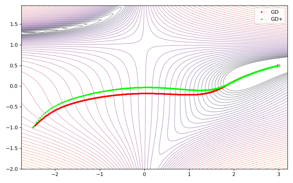
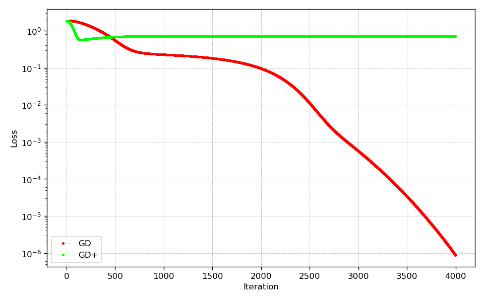
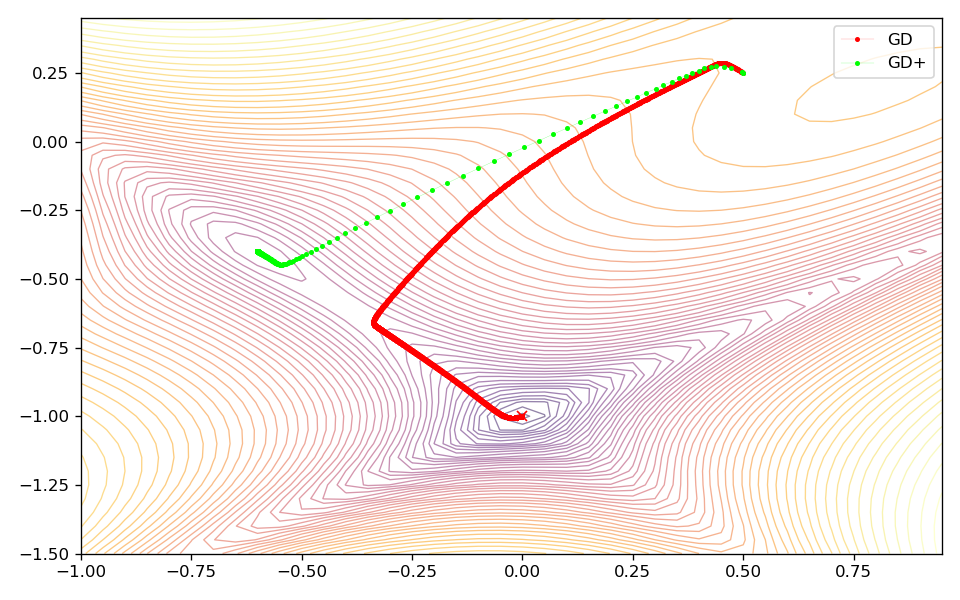
For the experiments I used the Rosenbrock, Beale, and the Goldstein-Price test functions to test gradient descent with and without weight extrapolation. These test function are often used to test the general performance of optimization algorithms. I used Adam as the gradient descent optimizer. In order to determine an optimal learning, a grid search was performed beforehand for all three test functions. For the evaluation of both approaches the error defined as the squared difference of the function’s value at the current position and the minimum’s position is used as the key metric.
The following learning rates have been found to work best for the Adam optimizer and the respective test function:
| Function | Rosenbrock | Beale | Goldstein-Price |
|---|---|---|---|
| Learning rate | 1e-1 | 1e-2 | 1e-3 |
| $\Delta t$ | 1e-4 | 1e-4 | 1e-5 |
Parameter $\Delta t$ used by the extrapolator was determined empirically. In addition, $h=\eta$ was assumed for all experiments.
Results and Discussion
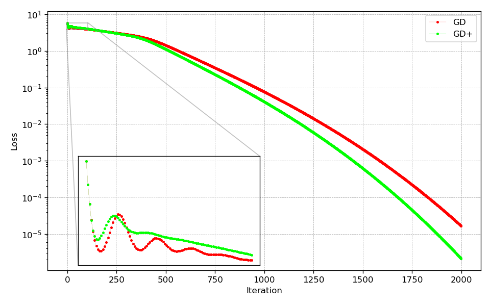
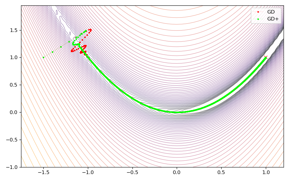
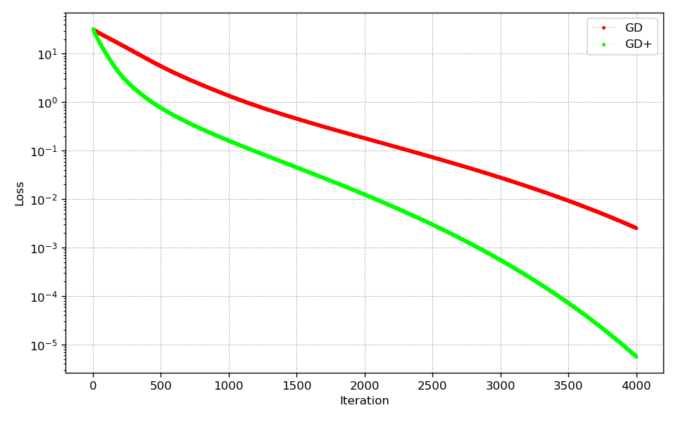
In case of the Rosenbrock and Beale test function, the extrapolator allows to converge faster to the global minimum. It is also noteworthy that in case of the Rosenbrock function, there are fewer oscillations at the beginning of the optimization allowing the optimizer to approach the minimum faster. However, it is important to note, that the additional extrapolation during optimization leads to the optimum being approached with less caution. This can be seen very clearly for the Beale test function, where this behavior leads to a less direct way to the minimum. In case of the Goldstein-Price function this behavior is even more pronounced, where the optimizer with extrapolation activated converges much faster at the beginning, but then gets stuck in a local minimum.
The results show that weight extrapolation can lead to faster convergence compared to the standard optimizer. However, experiments with more complex learning problems are necessary to better assess the proposed method.
Rosenbrock
Beale
Goldstein-Price
In case of more complex learning tasks, weight extrapolation as described in this post might work better for lager batch sizes as these result in better gradient approximations potentially leading to a smoother trajectories through parameter space. Deep learning systems that are able to process very large batch sizes could thus particularly benefit from this method. The same is true for smaller learning rates as these allow to compute better approximations for the derivatives necessary for weight extrapolation. Of course, this in turn can greatly slow down the training of the machine learning model.
As seen in this post, the Taylor series expansion allows for higher-order formulations of weight extrapolation that might or might not work as well. Reasons for that can be that computation of higher-order terms can become numerically unstable. There might be a high volatility of $w(t)$ especially at the beginning of training making it difficult to extrapolate the weights. However, it is reasonable to assume that higher-order formulations can be used in later stages of the training where the gradient updates are potentially less volatile as in the beginning.
Conclusion
In this post I described a method that allows to leverage the information stored in past gradients to perform weight extrapolation steps to speed up gradient-based optimization. Despite the simplicity of the method, adding extrapolation steps to the optimization process shows promising results and might also work for more complex problems.
@misc{Fischer2021we,
  title={Gradient-based Weight Extrapolation},
  author={Fischer, Kai},
  howpublished={\url{https://kaifishr.github.io/2021/09/05/weight-extrapolation.html}},
  year={2021}
}
You find the code for this project here.