Relevance Propagation with PyTorch
TL;DR: This post covers a basic, unsupervised, yet reasonably fast implementation of Layer-wise Relevance Propagation (LRP) in PyTorch and a novel relevance filter for crisper heatmaps.
Introduction
Layer-wise relevance propagation (LRP, Bach et al., Montavon et al.) helps us to identify input features that were relevant for network’s classification decision. Not long ago I posted an implementation for Layer-wise Relevance Propagation with Tensorflow on my blog where I also went into some of the theoretical underpinnings of LRP.
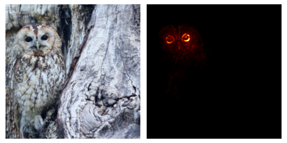

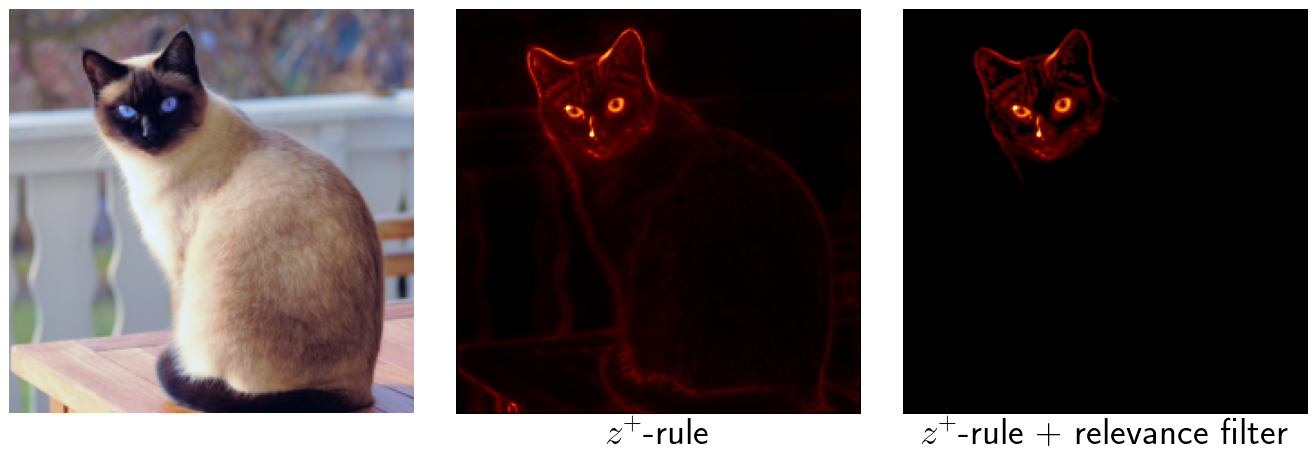
Figure 1: Layer-wise relevance propagation highlights input features that were dicisive for the network’s classification decision. It looks like the face or the eyes of the animals are particularly relevant for the network’s classification decision.
This post presents a very basic and unsupervised implementation of LRP in PyTorch for VGG networks from PyTorch’s Model Zoo. I also added a novel relevance propagation filter to this implementation resulting in much crisper heatmaps and far better relevance assignment. To the best of my knowledge, this method has not been published before. If you want to use it, please don’t forget to cite this post.
I have used this tutorial as well as a publication from Bach et al. and Montavon et al. as a starting point for my implementation. Both, the tutorial and the publications propose performing relevance propagation differently depending on the layer’s position in the network. There are also several hyperparameters involved depending on which rule is used to redistribute the relevance scores to the lower-layer neurons.
Since I am not a friend of hyperparamters myself, I implemented a version that comes without hyperparameters and where relevance scores are decomposed according to a single rule. I tried to make the code easy to understand as this implementation is primarily intended to get you started with LRP. I also focused a bit on modularity allowing the code to be easily extensible, which should help to use it for other projects.
Method
Relevance Assignment
Starting at the ouput layer, layer-wise relevance propagation assigns relevance scores to each of the network’s activations according to some relevance propagation rule until the input is reached. The neuron’s relevance is computed according to the following formula:
\begin{equation} \label{eq:lrp} R_i^{(l)} = \sum_j \frac{a_i w_{ij}}{\sum_{i’} a_{i’} w_{i’j}} R_j^{(l+1)} \end{equation}
Equation \eqref{eq:lrp} describes how relevance scores are being distributed in fully connected layers. $R_{i}^{(l)}$ and $R_j^{(l+1)}$ represent the relevance scores of neuron $i$ and $j$ in layer $(l)$ and $(l+1)$, respectively. Here, $(l)$ refers to the layer that is closer to the input, while layer $(l+1)$ is closer to the network’s output. $a_{i}$ represents the $i$th neuron’s activation and $w_{ij}$ stands for the weight connecting neurons $i$ and $j$ of layers $(l)$ and $(l+1)$.
In my implementation I use a slightly different version of the formula above, where only the positive weights are considered for the propagation of relevance. This rule is also know as the $z^+$-rule:
\begin{equation} \label{eq:zplus} R_i^{(l)} = \sum_j \frac{a_i w_{ij}^+}{\sum_{i’} a_{i’} w_{i’j}^+} R_j^{(l+1)} \end{equation}
As an aside, you may have noticed that Equation \eqref{eq:lrp} does not use the bias term in the denominator. This has to do with the fact that by adding the bias, the strength of the relevance signal does not remain constant at 1 (principle of relevance conservation). This problem can be solved by introducing an additional term in the numerator. This term expresses that the bias affects each neuron contribution equally.
\begin{equation} \label{eq:lrpWithBias} R_i^{(l)} = \sum_j \frac{a_i w_{ij} + \frac{b_{j}}{n}}{\sum_{i’=1}^n a_{i’} w_{i’j} + b_{j}} R_j^{(l+1)} \end{equation}
Since I noticed that adding the bias term has no particular effect on the quality of the heatmaps, I did not include it in my implementation. Aside over.
Relevance Computation
For the actual implementation, relevance propagation as shown in Equation \eqref{eq:lrp} can be divided into four separate steps. This can be seen better if Equation \eqref{eq:lrp} is rewritten as follows:
\begin{equation} \label{eq:lrp2} R_i^{(l)} = \color{orange}{\boxed{\color{black}{a_{i}} \color{blue}{\boxed{\color{black}{\sum_j w_{ij}}\color{lime}{\boxed{\color{black}{\frac{R_{j}^{(l+1)}}{\color{red}{\boxed{\color{black}{\sum_{i’} a_{i’} w_{i’j}}}}}}}}}}}} \end{equation}
$\color{red}{\boxed{\text{Step 1}}}$
The first step consists of a forward pass (here, omitting the bias term) in which we compute the total preactivation mass flowing from all neurons in layer $(l)$ to neuron $j$ in layer $(l+1)$. Thus we compute for every neuron $j$ in layer $(l+1)$:
\begin{equation} \label{eq:step1} \forall j: z_{j} = \sum_{i’} a_{i’} w_{i’j} \end{equation}
$\color{green}{\boxed{\text{Step 2}}}$
The second step consists of an element-wise division of relevance scores $R_{j}$ in layer $(l+1)$ by the preactivations $z_{j}$ computed in Step 1. This step ensures that the contributions of each neuron are put in proportion to the total contribution of all neurons. This step also ensures, that the relevance scores do not blow up while backpropagating the relevance scores and that the total relevance remains constant at 1. For every neuron $j$ in layer $(l+1)$ we compute:
\begin{equation} \label{eq:step2} \forall j: s_{j} = \frac{R_{j}^{(l+1)}}{z_{j}} \end{equation}
$\color{blue}{\boxed{\text{Step 3}}}$
Step three can be interpreted as a backward pass. For each neuron $i$ in layer $(l)$ we compute:
\begin{equation} \label{eq:step3} \forall i: c_{i} = \sum_{j} w_{ij} s_{j} \end{equation}
$\color{orange}{\boxed{\text{Step 4}}}$
The last step computes the final contributions of each neuron $i$ in layer $(l)$ to all neurons $j$ in layer $(l+1)$. To do this we weight the interim result from step 3 by the neuron’s activation $a_{i}$. Thus, for each neuron $i$ in layer $(l)$ we compute the element-wise product:
\begin{equation} \label{eq:step4} \forall i: R_{i}^{(l)} = a_{i} c_{i} \end{equation}
Gradient-based Relevance Computation
Redistributing relevance scores can become somewhat tedious for more complex mappings such as convolutional operations. In such a case, decomposing relevance scores would require special functions that cannot be implemented without greater effort. However, one can rewrite Equation \eqref{eq:step3} by expressing $c_{i}$ as an element of a gradient in the space of input activations $\mathbf{a}$ where $s_{j}$ is treated as a constant. We can rewrite Equation \eqref{eq:step3} into
\[\begin{equation} \begin{aligned} \label{eq:step3Gradient} c_{i} &= \sum_{j} w_{ij} s_{j} \\ & = \sum_{j} s_{j} \frac{\partial}{\partial a_{i}} \Big( \sum_{i'} a_{i'} w_{i'j}\Big)\\ & = \frac{\partial}{\partial a_{i}} \sum_{j} s_{j} z_{j}(\mathbf{a}; \mathbf{w})\\ & = \Big[\nabla \Big( \sum_{j} s_{j} z_{j}(\mathbf{a}; \mathbf{w}) \Big) \Big]_i \end{aligned} \end{equation}\]The gradient $\nabla f(\mathbf{a})$ in Equation \eqref{eq:step3Gradient} can be computed efficiently via automatic differentiation using PyTorch’s autograd engine. However, although this method is very convenient to implement, it can also be very slow and memory-hungry compared to a direct (i.e., gradient-free) implementation when possible.
The following code snippets are an example of relevance propagation through a linear layer. The first implementation is based on gradients. The second one is a direct implementation.
def lrp_gradient(layer: torch.nn.Linear, a: torch.tensor, r: torch.tensor) -> torch.tensor:
    eps = 1.0e-05
    z = layer.forward(a) + eps
    s = (r / z).data
    (z * s).sum().backward()
    c = a.grad
    r = (a * c).data
    return r
def lrp_manually(layer: torch.nn.Linear, a: torch.tensor, r: torch.tensor) -> torch.tensor:
    eps = 1.0e-05
    z = layer.forward(a) + eps
    s = r / z
    c = torch.mm(s, layer.weight)
    r = (a * c).data
    return r
In my tests with an RTX 2080 Ti and a linear layer mapping from 512 to 256 features the gradient-based approach was about five times slower.
Implementation
To generate an LRP model, the first step is to parse the original network’s operations. These operations create the first part of the LRP model. Then for each layer of the original model the corresponding LRP layer is added to the LRP model in reverse order. Thus, for every layer in the original network, there exists a corresponding LRP layer that inherits from the nn.Module class. Below I show exemplary the LRP counterpart of the convolution 2D layer. The relevance filter in the forward() method is optional but highly recommended ;)
class RelevancePropagationConv2d(nn.Module):
    """Layer-wise relevance propagation for 2D convolution.

    Optionally modifies layer weights according to propagation rule. Here z^+-rule

    Attributes:
        layer: 2D convolutional layer.
        eps: a value added to the denominator for numerical stability.

    """

    def __init__(self, layer: torch.nn.Conv2d, mode: str = "z_plus", eps: float = 1.0e-05) -> None:
        super().__init__()

        self.layer = layer

        if mode == "z_plus":
            self.layer.weight = torch.nn.Parameter(self.layer.weight.clamp(min=0.0))
            self.layer.bias = torch.nn.Parameter(torch.zeros_like(self.layer.bias))

        self.eps = eps

    def forward(self, a: torch.tensor, r: torch.tensor) -> torch.tensor:
        r = relevance_filter(r, top_k_percent=1.0)
        z = self.layer.forward(a) + self.eps
        s = (r / z).data
        (z * s).sum().backward()
        c = a.grad
        r = (a * c).data
        return r
Generating the actual LRP model then consists of only three lines of code:
model = torchvision.models.vgg16(pretrained=True)
lrp_model = LRPModel(model)
r = lrp_model.forward(x)
The presented implementation for relevance propagation is completely unsupervised. This means, that we do not use the input’s ground truth label as the starting point for the relevance propagation. At least in my tests, I found that starting relevance propagation from the true label (i.e., setting the class’ output activation and therefore the relevance to 1) had no significant effect on the resulting heatmap.
Relevance Filter
I have found that a very effective way of directing relevance scores to important features in input space is by using a filter that allows only the k% largest relevance scores to propagate to the next layer.
The idea for a relevance filter came from the assumption that a part of the activation signal and thus also the relevance signal are noise. The hypothesis is then that noise is more likely to be associated with small activations / relevance values. Thus, by filtering out small relevance values, the resulting heatmap should also become more focused on relevant features leading to much crisper heatmaps.
The code below shows the idea of a relevance filter implemented in PyTorch.
def relevance_filter(r: torch.tensor, top_k_percent: float = 1.0) -> torch.tensor:
    """Filter that allows largest k percent values to pass for each batch dimension.

    Filter keeps largest k% entries of a tensor. All tensor elements are set to
    zero except for the largest k % values. Here, k = 1 means that all relevance
    scores are passed on to the next layer.

    Args:
        r: Tensor holding relevance scores of current layer.
        top_k_percent: Proportion of top k values that is passed on.

    Returns:
        Tensor of same shape as input tensor.

    """
    assert 0.0 <= top_k_percent <= 1.0

    if top_k_percent < 1.0:
        size = r.size()
        r = r.flatten(start_dim=1)
        num_elements = r.size(-1)
        k = int(top_k_percent * num_elements)
        assert k > 0, f"Expected k to be larger than 0."
        top_k = torch.topk(input=r, k=k, dim=-1)
        r = torch.zeros_like(r)
        r.scatter_(dim=1, index=top_k.indices, src=top_k.values)
        return r.view(size)
    else:
        return r
As you can probably guess, the disadvantage of such a filter is that it is still relatively expensive due to the sorting of all relevance values. This is especially pronounced for convolutional layers, which can have a large number of activations.
Qualitative Results
In this section, I’ll briefly show a few results generated with the implementation presented in this post. In addition, I want to compare layer-wise relevance propagation without and with an additional relevance filter. As a baseline, I’ll use the example image from Montavon’s tutorial showing an old castle in the background of a busy street, with the corresponding LRP heatmap generated with several different relevance propagation rules and hyperparameters.

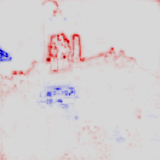
Figure 2:
Reference example from
Montavon's tutorial.
In Figure 2 we see that image regions associated with the Castle have been correctly identified as relevant for the network’s prediction. We can also observe negative relevance scores (blue) that are associated with part of a roof or the traffic sign. These regions had a negative effect on the output neuron that is connected to the castle class.
I have already mentioned, that I kept the implementation simple. So there is only one propagation rule, namely the $z^+$-rule that comes without any hyperparamters and only generates positive relevance scores in the range between 0 and 1. Let’s see how this vanilla implementation performs in comparison without and with relevance filter.
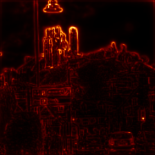

Figure 3:
Heatmaps generated with $z^+$-rule (left) and additional relevance filter (right).
On the left heatmap, it can be seen that compared to the reference heatmap, very similar areas have been marked as higly relevant for the network’s classification decision. However, it also appears that for this image, relevance scores are more widely distributed across the image.
Adding the relevance filter allowing only 5% of the largest relevance scores to propagate to the next layer, a significantly better focus of relevance on the castle is visible. Other areas of the heatmap turn almost completely black with activated filter. Even previously highly activated areas, such as the traffic light in the bottom right corner, are no longer relevant.
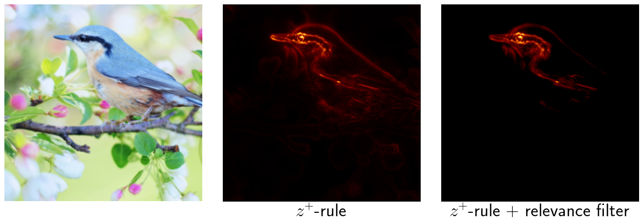
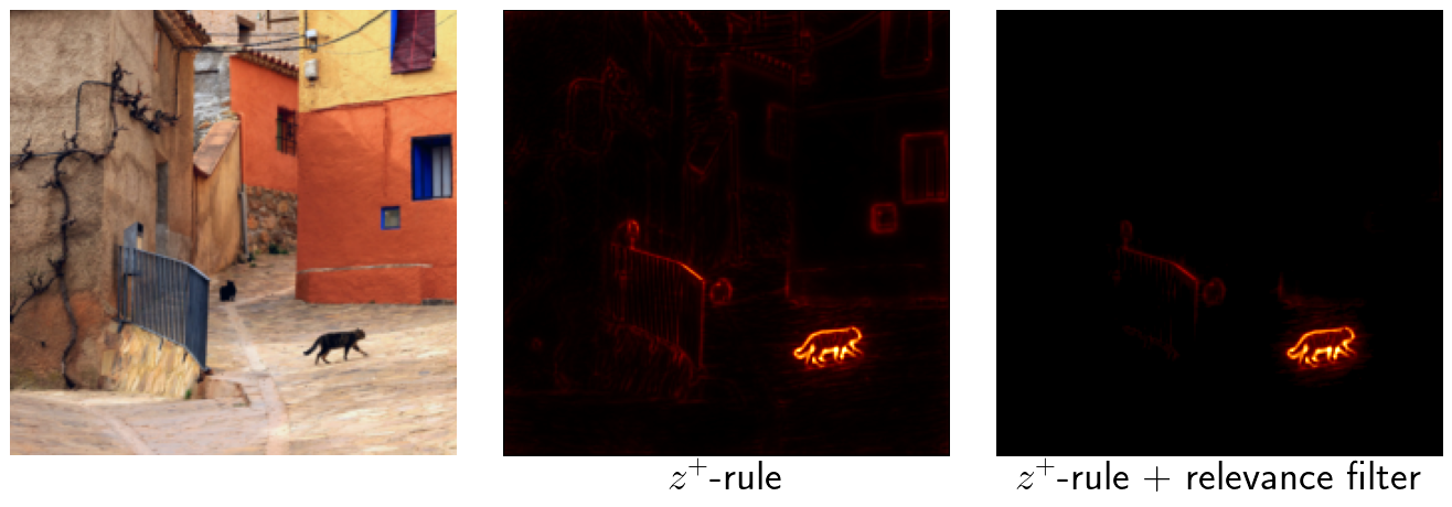
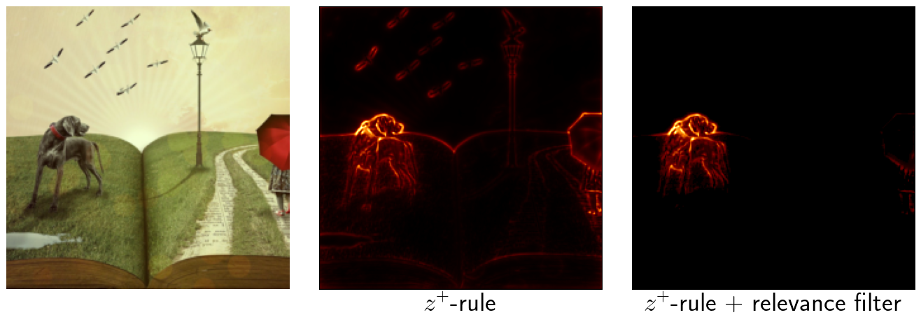
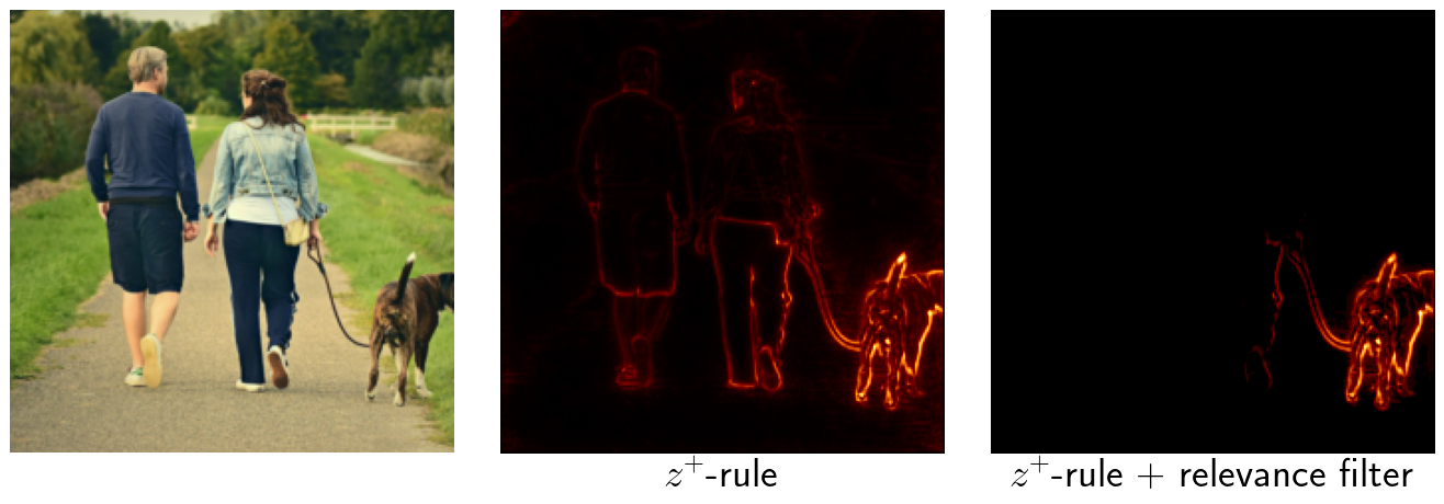
The following batch of images shows more results for different classes. The heatmap in the middle was created with the $z^+$-rule without further modifications. For the heatmap on the right, a relevance filter has been added suppressing 95% of the smallest relevance scores in each linear and convolutional layer.


Discussion and Outlook
The results show that adding a simple relevance filter can help to create better looking heatmaps that allow to make significantly better statements on the relevance of objects in the image.
There are some open points how the implementation can be further imporved. First, the implementation should be more model agnostic. Here, implementing all network operations using the gradient trick would be an important step in this direction. Second, one would have to think about how to get a list with the activations of all operations of the original network. I tried using forward hooks but was not able to extract the activations if a torch function such as torch.relu, torch.flatten, etc., was called during the forward pass.
Citation
@misc{Fischer2021rpp,
  title={Relevance Propagation with PyTorch},
  author={Fischer, Kai},
  howpublished={\url{https://kaifishr.github.io/2021/12/15/relevance-propagation-pytorch.html}},
  year={2021}
}
You find the code for this project here.