Training Neural Networks using Genetic Algorithms
Introduction
This post covers the topic of training artifical neural networks using genetic algorithms. An interesting aspect of this approach is that you must have never heard of the backpropagation gradient descent algorithm to train (small) neural networks. In a previous post I trained a simple classifier on the MNIST and Fashion-MNIST dataset using a genetic algorithm. There you’ll also find more information on evolutionary algorithms and genetic optimization.
Even though genetic optimization is by no means a worthy alternative to the optimization based on gradient descent, it is interesting to investigate the possibilities and properties of neural networks that were trained with these kind of algorithms.
In this post we’ll investigate the impact of different crossover operations, weight mutation rates, weight update rates, and layer-wise weight update schemes on the network’s performance. We’ll evaluate the network’s ability using two simple classification problems.
Methods
The various methods used for optimizing neural networks using genetic methods are discussed below. In order to determine the effectiveness of more advanced optimization methods, a baseline fully connected neural network trained with a vanilla genetic optimization method is used for comparsion. For the baseline model, a mutation rate of \(0.01\) and mutation probability \(0.1\) were used. In this post the following general conditions apply: During the optimization, agents cannot live for more than one period and crossover operations will only be carried out with the two best agents.
Network and Parameter Initialization
The network’s structure will be defined using a Python tuple consisting of the number of neurons of the input, hidden, and output layer(s).
network_layers = (n_input, 32, 32, 32, n_output)
Now, we can initialize the network’s trainable parameters stored in W and B. This implementation uses a method proposed by Kaiming He et al.. The weights of layer l are drawn from a normal distribution with zero mean and standard deviation of \(\sqrt{\frac{2}{n_l}}\), i.e., \(w_{ij}^{(l)} \sim \mathcal{N} (0, \sqrt{\frac{2}{n_l}})\). Biases are set to zero. This initialization scheme can be implemented with Python as follows
def kaiming(network_layers, l):
    return np.random.normal(size=(network_layers[l], network_layers[l+1])) \
           * np.sqrt(2./network_layers[l])
The networks’ weights can be initialized for the entire population at one go:
W = [[kaiming(network_layers, l) for l in range(n_layers-1)] \
    for p in range(n_agents)]
B = [[np.zeros((network_layers[l+1])) for l in range(n_layers-1)] \
    for p in range(n_agents)]
Here, n_agents represents the number of networks or the population size and n_layers represents the length of the tuple network_layers representing the network’s number of layers.
Local Weight Update Schemes
The essential ingredient of an evolutionary algorithm is the mutation operation. In fact, one could say that the mutation operation is all that is necessary to train any neural network, given enough time and computational resources. Generally speaking, genetic optimization is all about random mutation but non-random surviving.
The mutation rate determines how much a weight is changed and is comparable to the learning rate that you can find in many other optimization algorithms such as the workhorse algorithm SGD. The mutation rate itself is in the range between \((0, \infty)\). However, it must be added that small mutation rates are biologically and physically more plausible.
In real biological systems, mutations do not occur very often. Otherwise intelligent life would have had quite serious difficulties to evolve to the point we are today. This fact is reflected by the mutation probability. The mutation probability determines the chance that a mutation operation is performed on a weight. As the name indicates, this parameters lies between \(0\) and \(1\).
For a population of size n_agents of fully connected neural networks with n_layers per network with weights W, and biases B a simple mutation operation can be implemented as follows:
W = [[W[p][l] \
    + np.random.uniform(-mutation_rate, mutation_rate, size=W[p][l].shape) \
    * (np.random.random(W[p][l].shape) < mutation_prob) \
    for l in range(n_layers-1)] for p in range(n_agents)]
B = [[B[p][l] \
    + np.random.uniform(-mutation_rate, mutation_rate, size=B[p][l].shape) \
    * (np.random.random(B[p][l].shape) < mutation_prob) \
    for l in range(n_layers-1)] for p in range(n_agents)]
Global Weight Update Schemes
Due to the interdependence of the network’s weights or rather the impact of lower-layer computations on deeper-layer data representations, random changes of the network’s weights can cause cascades of erroneous signals that propagate through the network. Thus, random mutations of weights can cause errors of feature representation that propagate through the network and thus makes them difficult to train using the genetic approach. This leads to the effect that larger networks (many weights and layers) are much more difficult to train with the genetic approach. For this reason we’ll compare two different weight update schemes which take that behavior into account against the weight update scheme that optimizes the weights of all layers simultaneously.
Random Layer-wise Weight Update
This approach genetically modifies in a random manner one set of weights per optimization step. One set of weights represent the trainable parameters connecting two layers. For every network a different layer is selected. From all global weight update schemes, this approach makes the fewest assumptions and can be implemented as follows
for p in range(n_agents):
    l = np.random.randint(n_layers-1, size=1))
    W[p][l] = W[p][l] \
              + np.random.uniform(-mutation_rate, mutation_rate, size=W[p][l].shape) \
              * (np.random.random(W[p][l].shape) < mutation_prob)
    B[p][l] = B[p][l] \
              + np.random.uniform(-mutation_rate, mutation_rate, size=B[p][l].shape) \
              * (np.random.random(B[p][l].shape) < mutation_prob)
Cyclic Layer-wise Weight Update
The cyclic layer-wise weight update approach mutates only one layer per optimization step running either forward or backwards through the network. Variations such as mutating the same layer for several optimization steps are possible. Here the idea is to optimize the weights while freezing the weights of other layers.
l = n # here, n represents the current layer to be updated
for p in range(n_agents):
    W[p][l] = W[p][l] \
              + np.random.uniform(-mutation_rate, mutation_rate, size=W[p][l].shape) \
              * (np.random.random(W[p][l].shape) < mutation_prob)
    B[p][l] = B[p][l] \
              + np.random.uniform(-mutation_rate, mutation_rate, size=B[p][l].shape) \
              * (np.random.random(B[p][l].shape) < mutation_prob)
l -= 1
n = l % (n_layers - 1)
Crossover Operations
I’ll test two different crossover operations and compare the networks’ performance to the baseline network where crossover is disabled. The crossover operations combine the weights of different networks to create a new network configuration. All crossover operations have in common that they combine the genes of the two most successful agents to create a new agent. To do this, we have to get the index of the best two agents and store their chromosomes for further processing:
# Get indices of best two agents
idx_0, idx_1, *_= np.argsort(cost)

# Buffer weights of best two networks
W_0_tmp, B_0_tmp = np.copy(W[idx_0]), np.copy(B[idx_0])
W_1_tmp, B_1_tmp = np.copy(W[idx_1]), np.copy(B[idx_1])
The different crossover operations that will be tested are:
Average Crossover
The average crossover operation takes the weights of the two best networks and computes the element-wise average. This operation can be implemented as follows:
# Pooled weights crossover
W = [[0.5*(W_0_tmp[l] + W_1_tmp[l]) for l in range(len(layer_size)-1)] \
    for p in range(n_agents)]
B = [[0.5*(B_0_tmp[l] + B_1_tmp[l]) for l in range(len(layer_size)-1)] \
    for p in range(n_agents)]
Uniform Crossover
The uniform crossover operation creates a new network prototype by randomly selecting the weights of the two best networks. This operation can easily be implemented using a binary mask:
# Compute binary masks for crossover operation
W_mask = [[np.random.randint(2, size=W[p][l].shape) \
         for l in range(len(layer_size)-1)] for p in range(n_agents)]
B_mask = [[np.random.randint(2, size=B[p][l].shape) \
         for l in range(len(layer_size)-1)] for p in range(n_agents)]

# Different uniform crossover for every offspring
W = [[W_mask[p][l]*(W_0_tmp[l] - W_1_tmp[l]) + W_1_tmp[l] \
    for l in range(len(layer_size)-1)] for p in range(n_agents)]
B = [[B_mask[p][l]*(B_0_tmp[l] - B_1_tmp[l]) + B_1_tmp[l] \
    for l in range(len(layer_size)-1)] for p in range(n_agents)]
Neuron-wise Crossover
In their 1989 paper on genetic algorithms and neural networks, Montana et al. proposed a crossover operation that preserves the complete composition of a neuron by recombining complete sets of weights that are associated with a certain neuron in the network. This operation can be implemented as follows:
# Compute mask for neuron-wise crossover
mask = [[np.random.randint(2, size=B[p][l].shape) \
       for l in range(n_layers-1)] for p in range(n_agents)]

# Neuron-wise weight crossover
W = [[mask[p][l]*(W_0_tmp[l] - W_1_tmp[l]) + W_1_tmp[l] \
    for l in range(n_layers-1)] for p in range(n_agents)]
B = [[mask[p][l]*(B_0_tmp[l] - B_1_tmp[l]) + B_1_tmp[l] \
    for l in range(n_layers-1)] for p in range(n_agents)]
Layer-wise crossover
The resulting network of this crossover operation is composed of complete weight matrices of different agents that are merged to form a new agent. The probability of a weight matrix to be part of the new network is \(0.5\).
# Layer-wise weight crossover
W = [[W_0_tmp[l] if np.random.rand() < 0.5 else W_1_tmp[l] \
    for l in range(n_layers-1)] for p in range(n_agents)]
B = [[B_0_tmp[l] if np.random.rand() < 0.5 else B_1_tmp[l] \
    for l in range(n_layers-1)] for p in range(n_agents)]
Parameters
If not stated otherwise, the following parameters were used for all experiments:
n_agents = 4
mutation_rate = 0.01
mutation_prob = 0.1

n_input = 2
n_output = 2
network_layers = (n_input,) + 3*(32,) + (n_output,)
activation_fct = 'tanh'
batch_size = 256
Experiments and Results
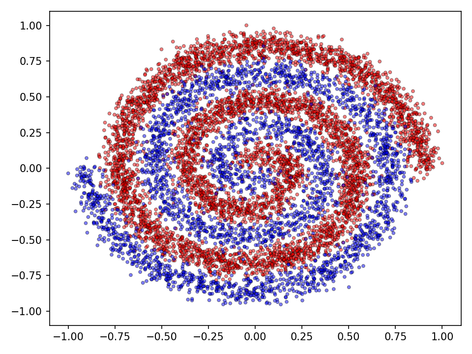
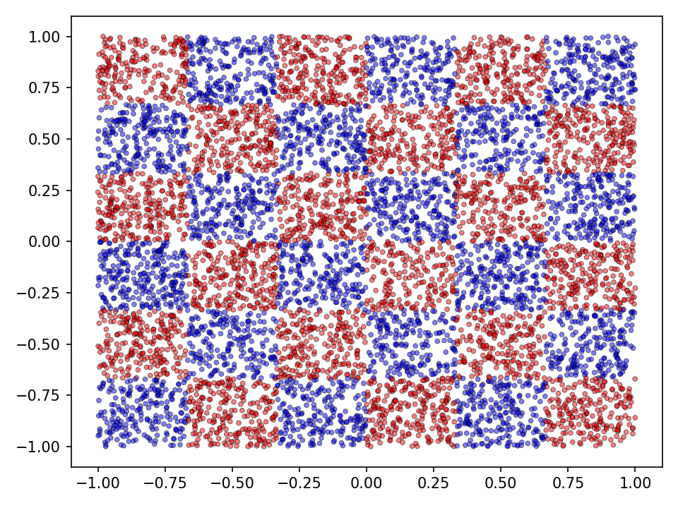
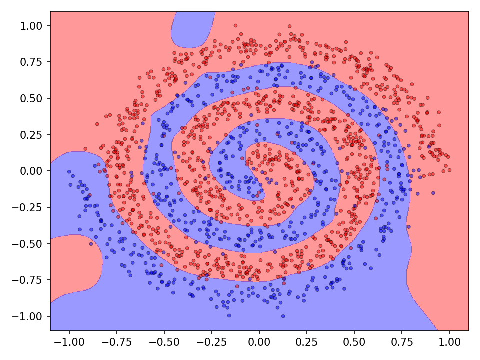
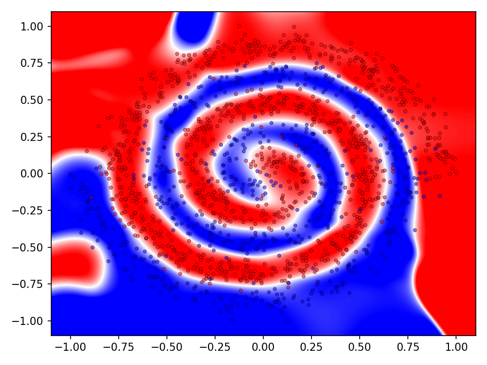
The following experiments compare the different methods introduced above and also serve for code validation. Two datasets consisting of two noisy intertwined spirals and a checkerboard distribution will serve as running examples (see Figures below). The training dataset consisted of \(20.000\) samples. The optimization was performed for \(10.000\) epochs which corresponds to \(1.560.000\)1 generations. For the qualitative evaluation I’ll visualize the classification (discrete) and prediction (continuous) landscape.
In both experiments the characteristics of increasingly sophisticated agents will be taken into account. This means, that more advanced types of mutation and crossover operations only become available after some time. This simulates more advanced or sophisticated agents. From an evolutionary biologically point of view we may assume that while organisms evolve their internal processes become more advanced. It can be reasonably assumed that more advanced agents are equiped with highly sophisticated internal mutation and crossover mechanisms. Very simple organisms, however, cannot perform these more advanced types of operations. Therefore, in both experiments, more advanced mutation and crossover operations become available after \(5.000\) epochs.
Experiment 1
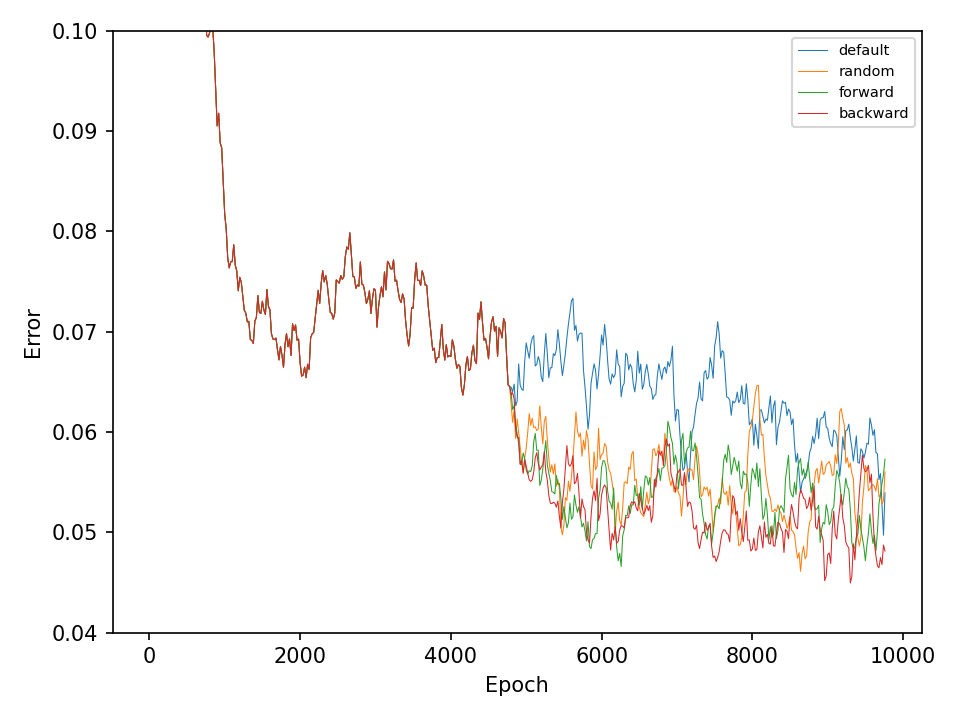
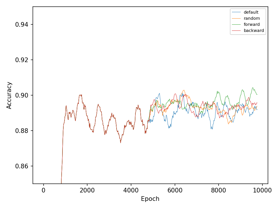
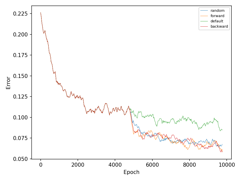
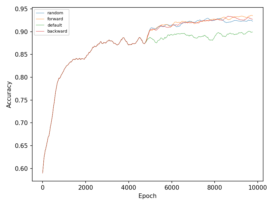
This experiment, compares the four types of mutation operations. The default operation, which mutates weights in all layers of the network, the random operation, which mutates only one layer of the network during every optimization step, and the forward and backward operations, which sequentially mutates one layer at every optimization step. The model in this experiment only uses different types of mutation operation during the optimization process and does not perform any type of crossover operation.
Let’s start with the results for the spiral dataset. The following two figures show the error and accuracy of the test set. The change to more advanced mutation operations has an immediate effect on the error rate. However, this difference cannot be maintained. The effect on the accuracy is very small.
The following visualization shows the classification and prediction landscape of the network using the random cycle mutation method. The network has learned in most cases to distinguish between the two classes. It is interesting to note, that the decision boundaries are very smooth and that there seems to be no tendency towards overfittig.
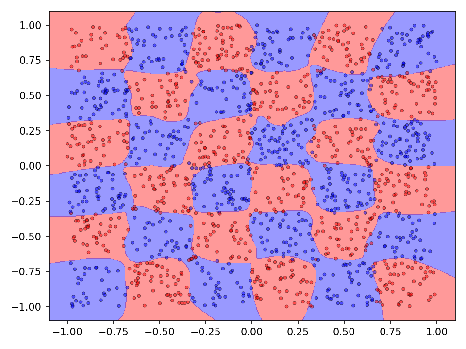
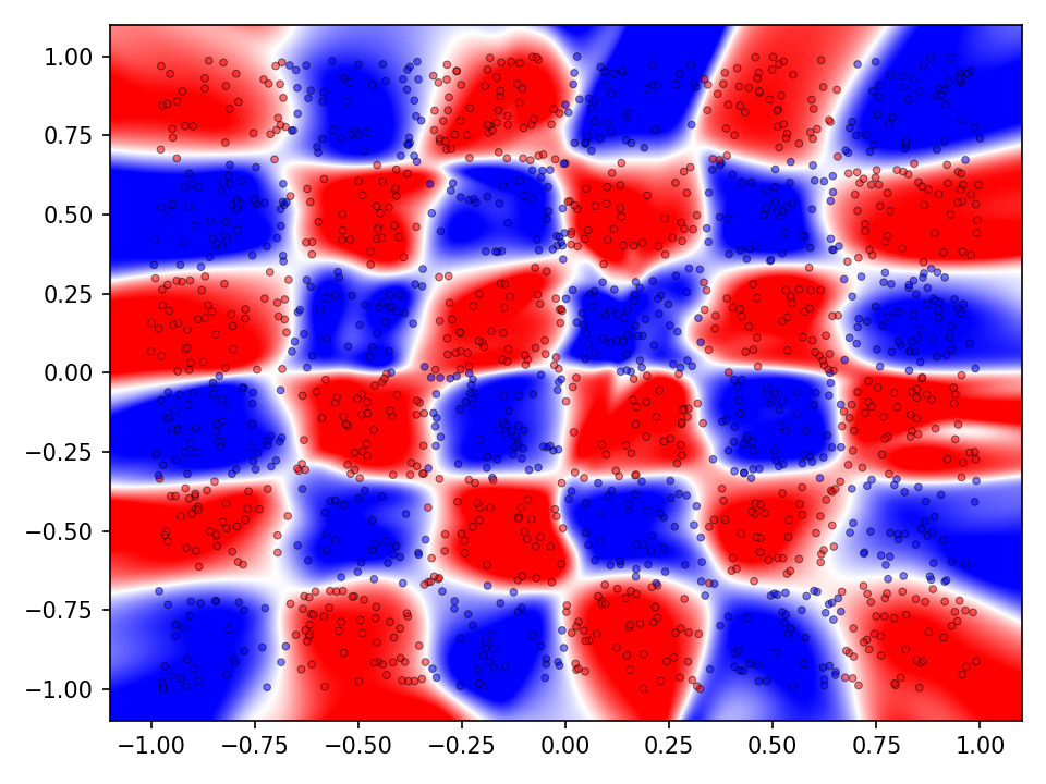
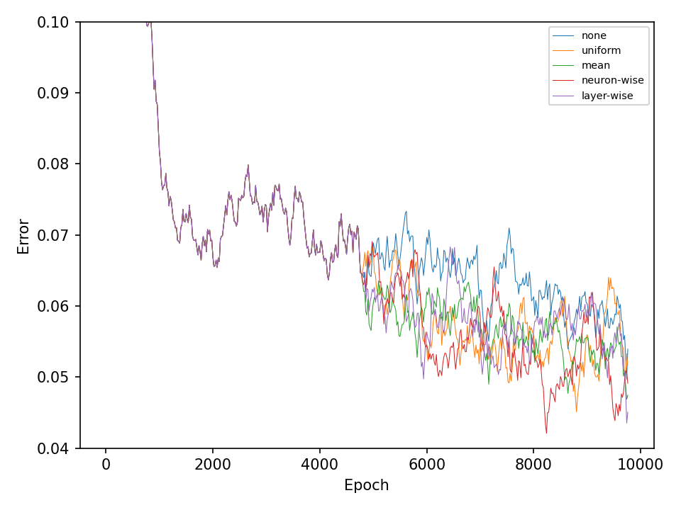
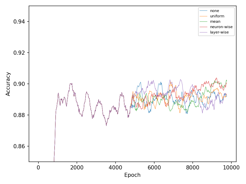
The difference between mutation operations is more pronounced in case of the checkerboard dataset. Here, a clear improvement after activating the more advaned mutation operation can be observed. However, all of the more advanced mutation operations seem to perform equally good and indicates that the network primarily benefits from fewer mutations that these operations entail.
Again, the network with random cycle mutation has been selected to visualize the results. Even though the accuracy on the test set is quite high, both, the classification as well as the prediction landscaped show that the decision boundaries are not optimal. Since the checkerboard dataset does not contain any noise, individual tiles of the same classes should not come into contact with each other. Both the error and accuracy indicate that the network has not yet converged and that a longer training time may improve the results.
Experiment 2
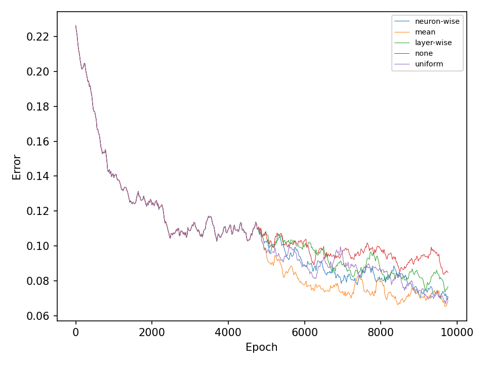
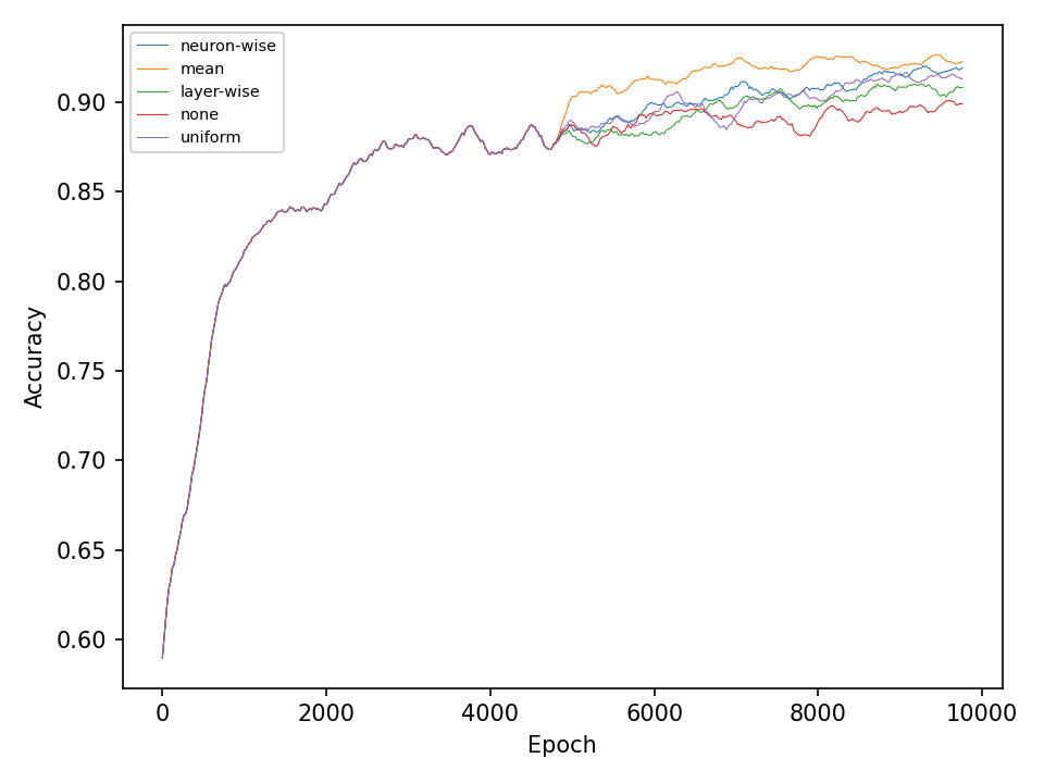
In the second experiment, I’ll compare four types of crossover operations to a baseline model without crossover. All models are equiped with the default mutation operation. The following two figures show the error and accuracy on the test dataset. For both datasets and at least in this experiment, there isn’t any clear superior crossover operation.
Conclusion
Simple deep neural networks can be trained using genetic algorithms. The results indicate, that for problems that are not too hard, simple genetic algorithms are sufficient to obtain good results. The results of the more difficult checkerboard dataset show, that the more advanced mutation methods are somewhat superior to the more simple implementations. However, further experiments are necessary for a better statement. It may be necessary to apply the presented optimization methods to harder problems in order to see more significant differences.
Check out my code on Github!
-
(20.000 [data points] / 128 [data points] / [optimization step]) * 10.000 [epochs] = 1.560.000 [generations] ↩