Neural Networks with Step Activation Functions
TL;DR: Neural networks equipped with step activation functions cannot be trained using a gradient based optimizer. This blog post shows that they can, however, be optimized using a genetic approach.
Introduction
In my last post I trained simple fully connected neural networks using evolutionary algorithms and compared different optimization schemes. This time the focus is on networks equipped with step activation functions that no longer allow gradient based optimization.
Modern optimization methods are based on the calculation of gradients in order to update the trainable parameters and to minimize the error of the network. For a weight \(w\) connecting two neurons \(j\) and \(k\) in the layers \(l\) and \(l-1\) of a fully connected neural network, the update rule is as follows
\[w^{(t+1)} = w^{(t)} - \eta \cdot \frac{\partial C}{\partial w^{(t)}}\]where \(w^{(t)}\) and \(w^{(t+1)}\) represent the old and the new updated weight, respectively. The learning rate of the algorithm is given by \(\eta\). The gradient for this weight, \(\frac{\partial C}{\partial w^{(t)}}\), is computed as follows
\[\frac{\partial C}{\partial w_{jk}^{(l,l-1)}} = \frac{\partial z_j^{(l)}}{\partial w_{jk}^{(l,l-1)}} \cdot \frac{\partial a_j^{(l)}}{\partial z_j^{(l)}} \cdot \frac{\partial C}{\partial a_j^{(l)}} = a_k^{(l-1)} \cdot h'(z_j^{(l)}) \cdot \frac{\partial C}{\partial a_j^{(l)}}\]This formula shows that the derivative of the activation function, \(h'(z_j^{(l)})\), is needed to calculate the gradient that is necessary to update the trainable parameter \(w\). This fact limits modern neural networks to activation functions whose derivative is not zero everywhere.
Functions where the derivative is always zero are for example the Heaviside, Sign or Floor activation functions. Thus, no gradients can be computed to update the network’s trainable parameters. However, there is genetic optimization than allows to use such types of activation functions in neural networks.
In this blog post I’ll focus on the use of step activation functions in fully connected neural networks and how well they can be used for classification tasks.
Methods
Step Activation Functions
For the experiments, I’m going to use different kinds of step activation functions and compare them to each other. For the discretization of continuous functions, the following piece of code will be used:
def discretize(x, discretization):
    return np.round(discretization * x) / discretization
The discretization parameter determines the number of discrete steps per unit. The following visualizations show the activation functions and their corresponding Python implementation.
Heaviside
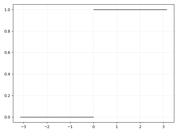
def heaviside(x):
    return np.heaviside(x, 0.0)
Floor
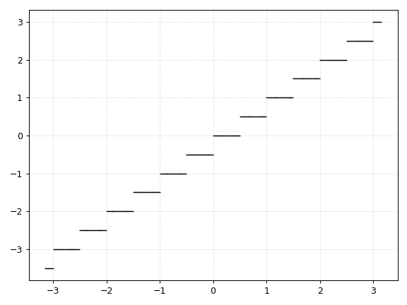
def dfloor(x, d):
    return np.floor(d * x) / d
However, this is an extension of the Floor function where the parameter d determines the number of steps per unit. As d approaches infinity, the above implementation of the Floor function becomes the identiy function \(f(x) = x\).
Discrete Relu
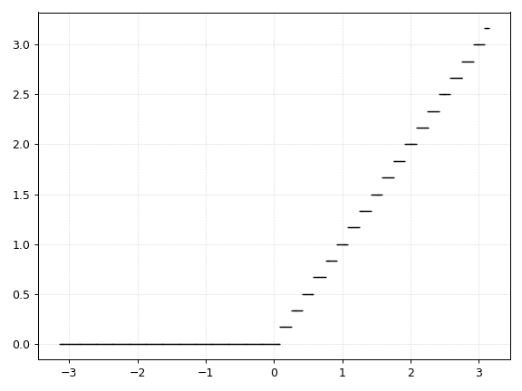
def drelu(x):
    return discretize(x * (x > 0.0))
The discrete Relu activation function is in fact just a special case of the Floor function.
Model Architecture and Parameters
If not stated otherwise, the following experimental setup was used for all experiments:
n_points = 10000

n_inputs = 2
n_outputs = 2
network_layers = (n_inputs,) + 3*(16,) + (n_outputs,)

n_agents = 4
batch_size = 256
mutation_rate = 0.01
mutation_prob = 0.01

mutation_type = 'random_cycle'
crossover_type = 'neuron_wise'
You can find more information about the terms mutation_rate, mutation_prob, mutation_type, and crossover_type in my last post. During the experiments, the discretization parameters of all activation functions were set to 1.
Experiments and Results
The performance of step activation functions is tested on three popular classification tasks: the moons, spirals and the checkerboard dataset.
The discrete classification landscape and the continuous prediction landscape for the respective dataset is visualized for the qualitative evaluation. For the quantitative evaluation, the loss and classification accuracy of the model is determined on the test dataset.
To get a better feeling of what function the network has learned, the model’s prediction is displayed beyond the known data domain.
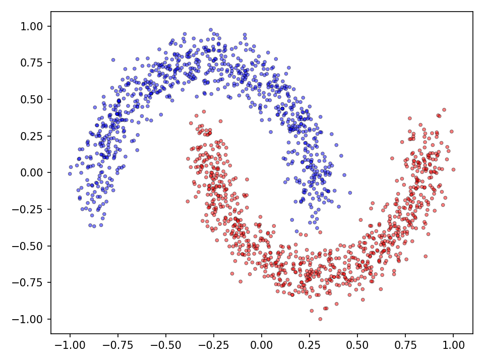
Moons
First the results for the moon dataset.
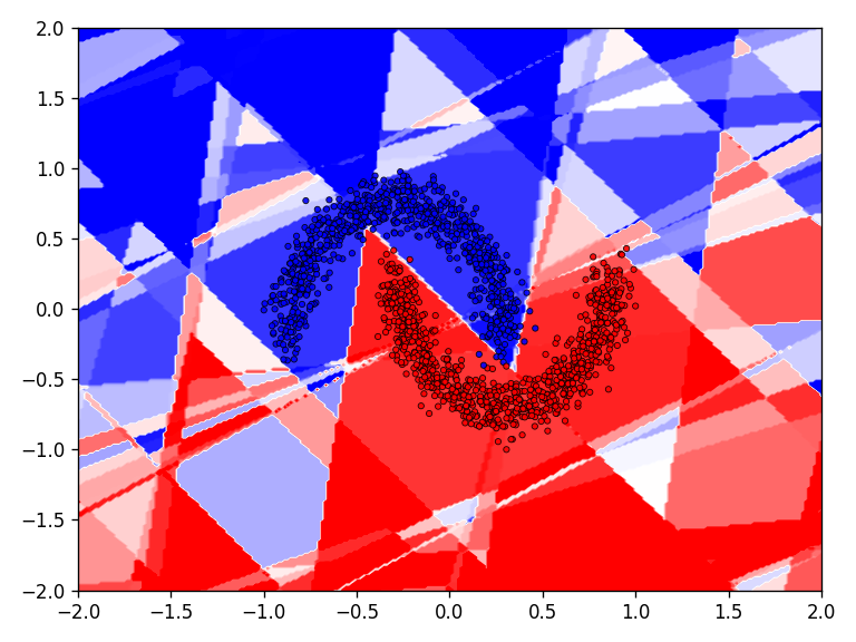
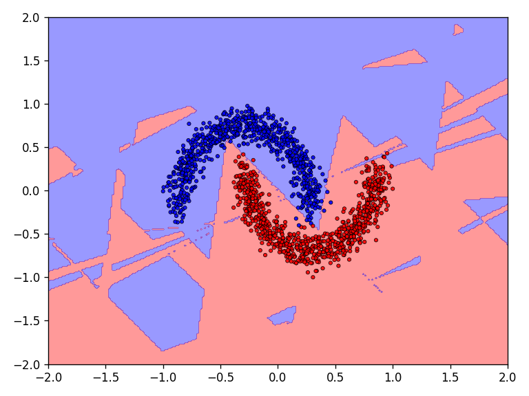

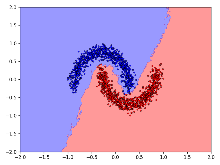
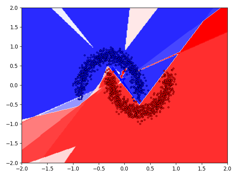

The qualitative results show that all tested functions have no major difficulties with the relatively simple moons dataset. This is also reflected in the results for the error and accuracy.

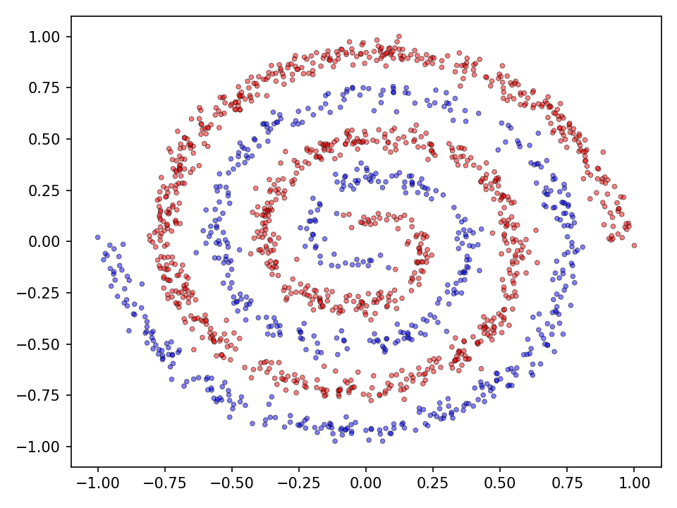
Spirals
Now the results for the somewhat more complex intertwined spirals dataset.
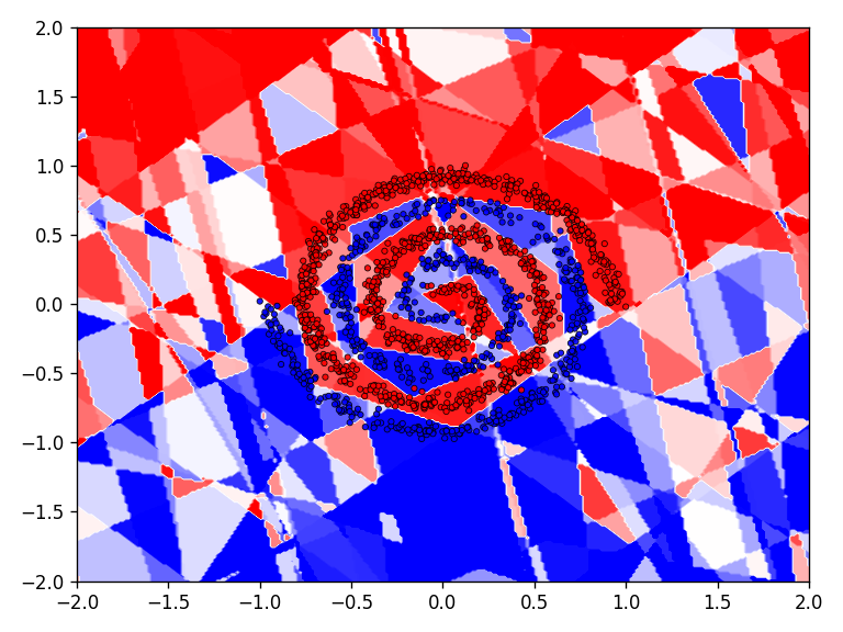

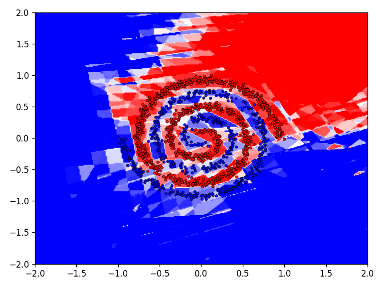
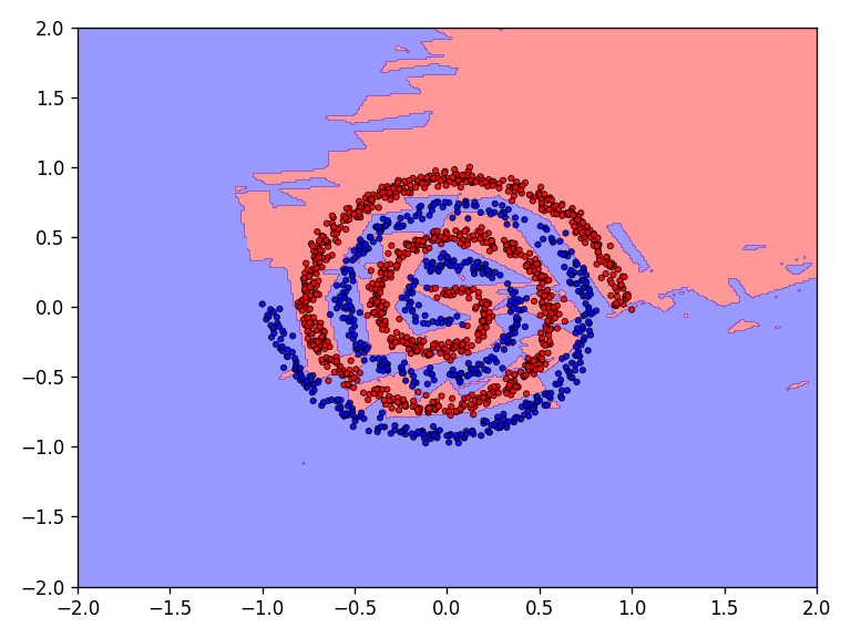


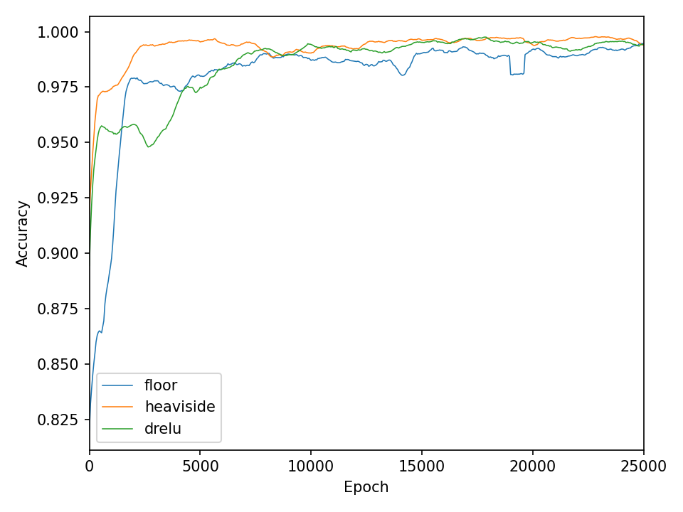
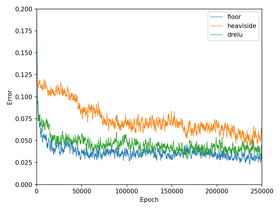
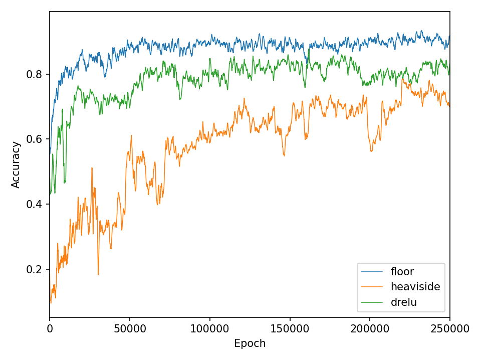
The qualitative results clearly show that the task is no longer so easy to accomplish for all functions. The network needs significantly more iterations to achieve reasonably good results. This is also reflected in the network’s loss and accuracy.
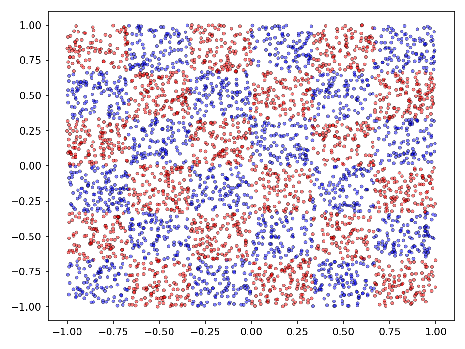
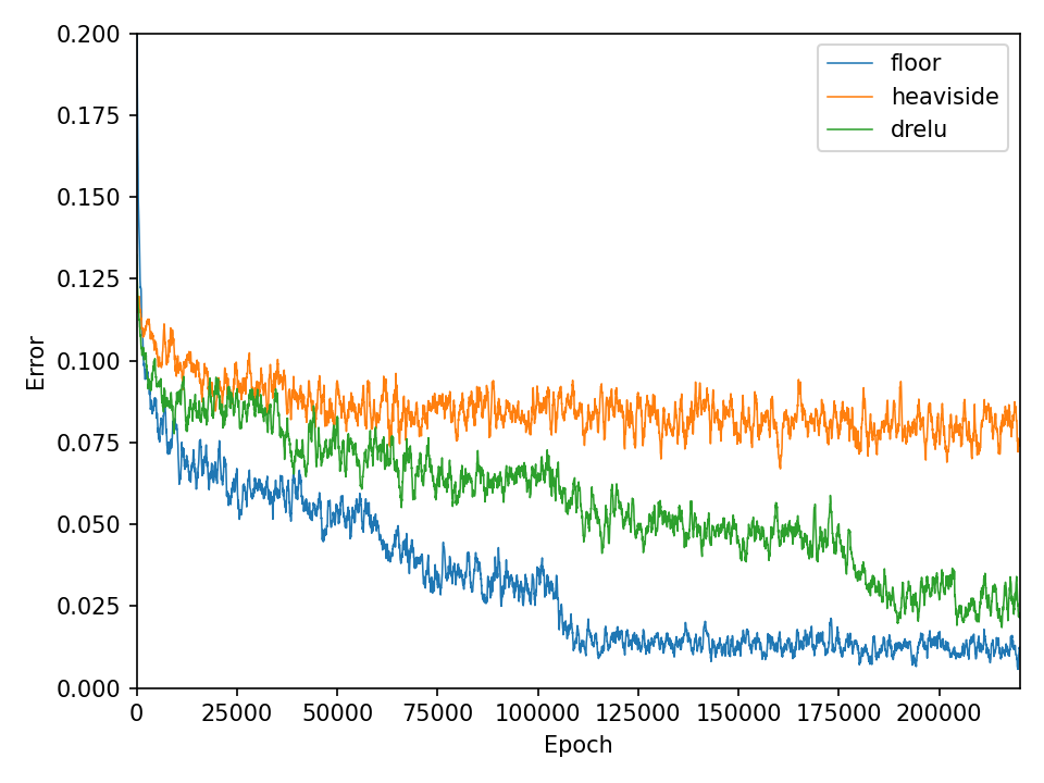
Checkerboard
Now the results for the checkerboard dataset.


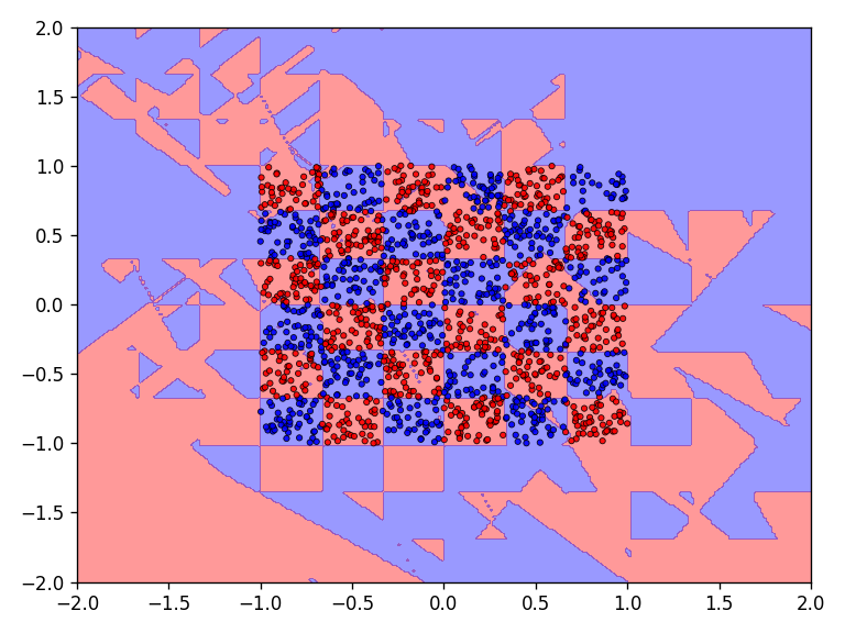

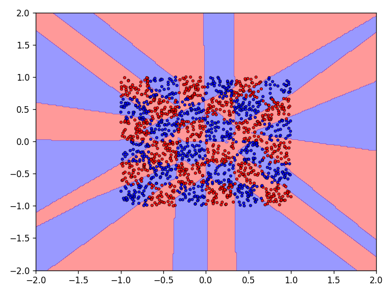
The results for the chessboard data set show clear differences in performance. The floor function converges by far the fastest and achieves high accuracy. It is also interesting to see that the model with the floor function generalizes very well beyond the data domain. This is not the case for the networks with the discrete Relu and the Heaviside function. The differences in performance are also apparent in the error and accuracy.

Conclusion
The results show that simple neural networks equipped with step activation functions and trained with the help of genetic optimization are quite capable of learning complex functions. It can be assumed that much more complex problems can be solved with larger networks.
You find the code for this project on Github. Check out my other posts on genetic optimization: here and here.